flowchart LR
    T[Time Domain] -->|FFT| F[Frequency Domain]
    F -->|Inverse FFT| T
Appendix B: Signal Processing Basics
Fundamentals for Audio and Sensor Data
This appendix covers signal processing concepts for LAB04 (Keyword Spotting), LAB10 (EMG), and LAB12 (Streaming).
Time Domain vs Frequency Domain
Time Domain
Signal amplitude over time:
Code
import numpy as np
import matplotlib.pyplot as plt

# Generate a signal: 5Hz + 20Hz components
fs = 1000  # Sampling rate
t = np.linspace(0, 1, fs)
signal = np.sin(2 * np.pi * 5 * t) + 0.5 * np.sin(2 * np.pi * 20 * t)

plt.figure(figsize=(10, 3))
plt.plot(t[:200], signal[:200])
plt.xlabel('Time (s)')
plt.ylabel('Amplitude')
plt.title('Time Domain Signal')
plt.grid(True)
plt.show()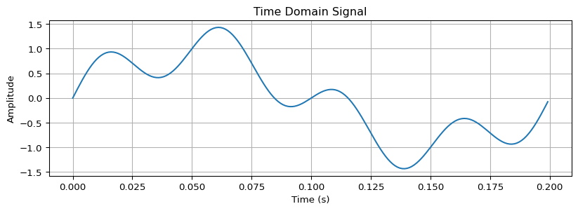
Frequency Domain
Signal components by frequency:
Code
from scipy.fft import fft, fftfreq

# Compute FFT
N = len(signal)
yf = fft(signal)
xf = fftfreq(N, 1/fs)

plt.figure(figsize=(10, 3))
plt.plot(xf[:N//2], np.abs(yf[:N//2]) * 2/N)
plt.xlabel('Frequency (Hz)')
plt.ylabel('Magnitude')
plt.title('Frequency Domain (FFT)')
plt.xlim(0, 50)
plt.grid(True)
plt.show()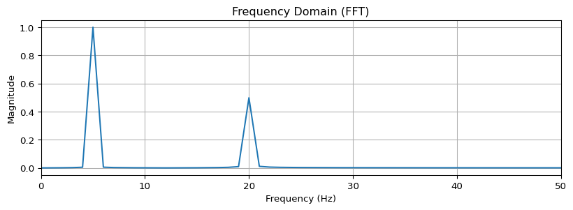
Filtering
Low-Pass Filter
Removes high frequencies (keeps slow changes):
Code
from scipy.signal import butter, filtfilt

def lowpass_filter(data, cutoff, fs, order=4):
    """Butterworth low-pass filter"""
    nyquist = fs / 2
    normalized_cutoff = cutoff / nyquist
    b, a = butter(order, normalized_cutoff, btype='low')
    return filtfilt(b, a, data)

# Apply 10Hz low-pass filter
filtered = lowpass_filter(signal, cutoff=10, fs=fs)

plt.figure(figsize=(10, 3))
plt.plot(t[:200], signal[:200], alpha=0.5, label='Original')
plt.plot(t[:200], filtered[:200], label='Filtered (10Hz LP)')
plt.xlabel('Time (s)')
plt.ylabel('Amplitude')
plt.legend()
plt.grid(True)
plt.show()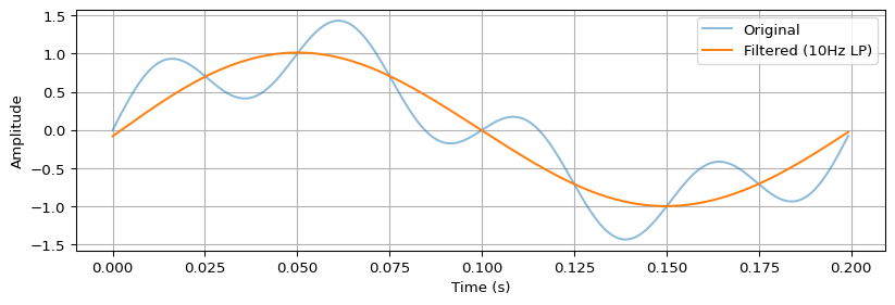
Band-Pass Filter
Keeps only frequencies in a range (used in EMG):
Code
def bandpass_filter(data, low, high, fs, order=4):
    """Butterworth band-pass filter"""
    nyquist = fs / 2
    low_norm = low / nyquist
    high_norm = high / nyquist
    b, a = butter(order, [low_norm, high_norm], btype='band')
    return filtfilt(b, a, data)

# EMG typically uses 20-450Hz band-pass
# emg_filtered = bandpass_filter(emg_signal, 20, 450, fs=1000)
Filter Frequency Response
Code
from scipy.signal import freqz

# Design filter
b, a = butter(4, 10/(fs/2), btype='low')

# Compute frequency response
w, h = freqz(b, a, worN=2000, fs=fs)

plt.figure(figsize=(10, 4))
plt.subplot(1, 2, 1)
plt.plot(w, 20 * np.log10(abs(h)))
plt.xlabel('Frequency (Hz)')
plt.ylabel('Magnitude (dB)')
plt.title('Magnitude Response')
plt.grid(True)
plt.xlim(0, 50)

plt.subplot(1, 2, 2)
plt.plot(w, np.unwrap(np.angle(h)))
plt.xlabel('Frequency (Hz)')
plt.ylabel('Phase (radians)')
plt.title('Phase Response')
plt.grid(True)
plt.xlim(0, 50)
plt.tight_layout()
plt.show()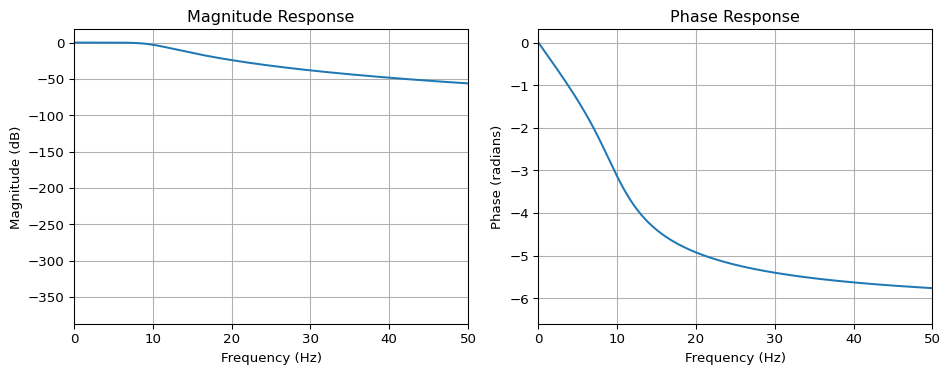
Spectrograms
Time-frequency representation:
Code
from scipy.signal import spectrogram

# Create a chirp signal (frequency changes over time)
t = np.linspace(0, 2, 2000)
chirp = np.sin(2 * np.pi * (5 + 20*t) * t)

# Compute spectrogram
f, t_spec, Sxx = spectrogram(chirp, fs=1000, nperseg=128)

plt.figure(figsize=(10, 4))
plt.pcolormesh(t_spec, f, 10 * np.log10(Sxx), shading='gouraud')
plt.ylabel('Frequency (Hz)')
plt.xlabel('Time (s)')
plt.title('Spectrogram')
plt.colorbar(label='Power (dB)')
plt.ylim(0, 100)
plt.show()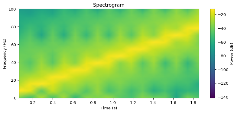
MFCCs for Audio
Mel-Frequency Cepstral Coefficients are used in keyword spotting:
Code
import librosa

# Load audio
y, sr = librosa.load('audio.wav', sr=16000)

# Compute MFCCs
mfccs = librosa.feature.mfcc(y=y, sr=sr, n_mfcc=40)

# Plot
plt.figure(figsize=(10, 4))
librosa.display.specshow(mfccs, sr=sr, x_axis='time')
plt.colorbar()
plt.title('MFCCs')
plt.show()
Why MFCCs?
- Mel scale: Mimics human hearing (logarithmic)
- Compact: ~40 coefficients vs thousands of FFT bins
- Robust: Less sensitive to noise than raw spectrograms
Windowing
Divide continuous signals into overlapping frames:
Code
def frame_signal(signal, frame_size, hop_size):
    """Split signal into overlapping frames"""
    frames = []
    for i in range(0, len(signal) - frame_size, hop_size):
        frames.append(signal[i:i + frame_size])
    return np.array(frames)

# Example: 25ms frames, 10ms hop
frame_size = int(0.025 * 1000)  # 25 samples at 1kHz
hop_size = int(0.010 * 1000)    # 10 samples

frames = frame_signal(signal, frame_size, hop_size)
print(f"Signal length: {len(signal)}, Frames: {frames.shape}")
Signal length: 1000, Frames: (98, 25)Window Functions
Code
from scipy.signal import windows

n = 64  # Window size

plt.figure(figsize=(10, 4))
plt.plot(windows.boxcar(n), label='Rectangular')
plt.plot(windows.hamming(n), label='Hamming')
plt.plot(windows.hann(n), label='Hann')
plt.plot(windows.blackman(n), label='Blackman')
plt.xlabel('Sample')
plt.ylabel('Amplitude')
plt.title('Window Functions')
plt.legend()
plt.grid(True)
plt.show()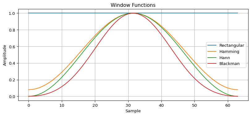
Feature Extraction
RMS (Root Mean Square)
Measures signal energy:
Code
def rms(signal):
    return np.sqrt(np.mean(signal**2))

# Example
print(f"RMS: {rms(signal):.4f}")
RMS: 0.7902Zero Crossing Rate
Counts sign changes (used in speech/music):
Code
def zero_crossing_rate(signal):
    return np.sum(np.diff(np.sign(signal)) != 0) / len(signal)

print(f"ZCR: {zero_crossing_rate(signal):.4f}")
ZCR: 0.0200Peak Detection
Find local maxima:
Code
from scipy.signal import find_peaks

# Find peaks
peaks, properties = find_peaks(signal[:200], height=0.5, distance=20)

plt.figure(figsize=(10, 3))
plt.plot(signal[:200])
plt.plot(peaks, signal[peaks], 'rx', markersize=10)
plt.xlabel('Sample')
plt.ylabel('Amplitude')
plt.title('Peak Detection')
plt.grid(True)
plt.show()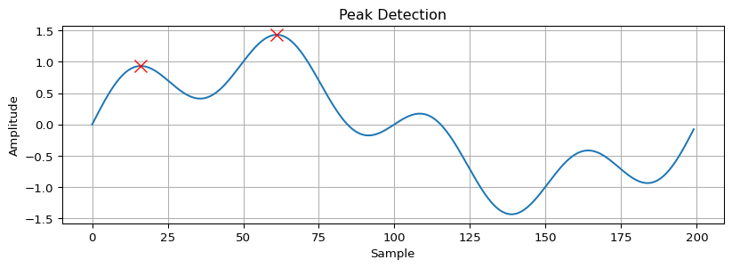
Quick Reference
| Concept | Function | Use Case |
|---|---|---|
| FFT | scipy.fft.fft() |
Frequency analysis |
| Low-pass | butter(..., 'low') |
Smooth sensor data |
| Band-pass | butter(..., 'band') |
EMG, audio |
| Spectrogram | scipy.signal.spectrogram() |
Audio classification |
| MFCCs | librosa.feature.mfcc() |
Keyword spotting |
| RMS | np.sqrt(np.mean(x**2)) |
Energy/amplitude |
Further Reading
- Think DSP - Free online book
- The Scientist and Engineer’s Guide to DSP - Comprehensive reference
- librosa Documentation - Audio processing