For detailed theoretical foundations, mathematical proofs, and algorithm derivations, see Chapter 11: Edge Device Profiling and Optimization in the PDF textbook.
The PDF chapter includes: - Detailed timing measurement theory and timer resolution analysis - Complete memory profiling methodology and tools - In-depth power measurement circuits and INA219 theory - Mathematical models for performance bottleneck identification - Comprehensive optimization strategies with theoretical justifications
Measure code execution time on microcontrollers using millisecond and microsecond timers
Profile memory footprint (SRAM/Flash/tensor arena) of TinyML applications
Measure power consumption and estimate battery life for typical workloads
Compare Float32 vs Int8 models in terms of size, latency, and accuracy
Apply targeted optimizations based on profiling results rather than guesswork
Theory Summary
Profiling transforms speculation into science. Edge devices have severe constraints—Arduino Nano 33 BLE offers 256 KB SRAM and runs at 64 MHz, compared to laptops with 16 GB RAM and 3+ GHz CPUs (a 60,000x memory gap and 50x speed gap). Without measurement, you cannot know if your ML model will fit, run fast enough for real-time requirements, or drain the battery in hours versus months.
Timing measurement uses millis() (1 ms resolution) for operations >10 ms and micros() (4 μs resolution on most boards) for fast operations. Critical insight: always discard the first run as warmup to eliminate cache-loading effects that can inflate latency 2-10x. Statistical benchmarking runs 50-100 trials to compute mean, standard deviation, min/max, and percentiles (p95, p99). High variance indicates inconsistent execution—often from interrupts, dynamic memory allocation, or unstable power supply.
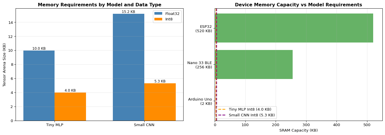
Memory profiling distinguishes three regions: (1) Flash stores compiled code and model weights (persistent, abundant at 1-4 MB), (2) SRAM holds variables, stack, heap, and TensorFlow’s tensor arena (volatile, scarce at 8-256 KB), (3) Tensor arena is the critical bottleneck—TensorFlow Lite Micro allocates this contiguous block for activation tensors during inference. Int8 quantization typically reduces both model size and arena requirements by 3-4x compared to Float32. The ESP32’s getMinFreeHeap() reveals peak memory usage—if this approaches zero, your application will crash unpredictably.
Power profiling uses INA219 current sensors or USB power meters to measure actual consumption. Key principle: average current determines battery life. For duty-cycled operation (wake periodically, run inference, sleep), compute weighted average: (I_active × t_active + I_sleep × t_sleep) / (t_active + t_sleep). Example: ESP32 deep sleep at 0.01 mA, active inference at 80 mA for 2 seconds per minute yields 2.68 mA average → 2000 mAh battery lasts 750 hours (31 days) versus 25 hours if continuously active. Optimization often targets duty cycling over raw inference speed.
Key Concepts at a Glance
Timing Functions: millis() for ms resolution (ops >10 ms), micros() for μs resolution (fast ops); both use unsigned long to handle overflow at 49 days / 71 minutes
Statistical Benchmarking: Discard first 1-5 runs (warmup), collect 50-100 samples, report mean ± std, min/max, p95/p99; high variance indicates instability
Compile-Time vs Runtime: Arduino IDE reports global variable usage (~15% SRAM for “hello world”) but misses dynamic allocations; runtime profiling via ESP.getFreeHeap() or freeMemory() shows actual usage
Int8 vs Float32: Quantization yields 3-4x model size reduction, 2.5-3x arena reduction, 3-5x speed improvement, <1% accuracy loss for most models
Power Measurement: INA219 sensor measures voltage and current via I2C; calculate energy/inference = V × I × t; estimate battery life = capacity / average_current
Optimization Decision Tree: Profile first → identify bottleneck (memory/latency/power) → apply targeted fix → profile again to verify; don’t optimize blindly!
Common Pitfalls
Reporting first-run latency: The initial inference is 2-10x slower due to cache warmup and lazy initialization. Always run 5+ warmup iterations before collecting timing data, or clearly label cold-start vs warm latency.
Ignoring standard deviation: Reporting only mean latency hides critical variance. A system with 50 ms ± 30 ms cannot meet a 60 ms deadline (p99 > 100 ms). Real-time systems care about worst-case (max or p99), not average.
Confusing compile-time and runtime memory: Arduino IDE reports 15% SRAM used, but runtime crashes when allocating tensor arena. Compile-time only counts global variables; dynamic allocations (stack growth, heap fragmentation) appear at runtime.
Insufficient power supply for measurement: USB ports provide 500 mA, but WiFi bursts draw 240 mA. Voltage sag causes clock jitter and timing measurement errors. Use stable 1A+ supply for accurate profiling.
Optimizing the wrong bottleneck: Speeding up inference 2x doesn’t help if deep sleep dominates battery life. Profile to find actual bottleneck: 60% time in memory allocation → fix memory, not computation. Measure before optimizing!
Quick Reference
Key Formulas
Battery Life with Duty Cycling\[
I_{\text{avg}} = \frac{I_{\text{active}} \cdot t_{\text{active}} + I_{\text{sleep}} \cdot t_{\text{sleep}}}{t_{\text{active}} + t_{\text{sleep}}}
\]
\[
\text{Battery Life (hours)} = \frac{\text{Capacity (mAh)}}{I_{\text{avg}} \text{ (mA)}}
\]
Energy Per Inference\[
E_{\text{inference}} = V \times I_{\text{active}} \times t_{\text{inference}} \quad \text{(in Joules or mJ)}
\]
Section 7: Float32 vs Int8 quantization comparison (pages 26-28)
Section 8: Complete profiling workflow example (pages 29-33)
Section 10: Case studies showing optimization decisions (pages 36-40)
Self-Assessment Checkpoints
Test your understanding before proceeding to the exercises.
Question 1: Your model’s first inference takes 180ms but subsequent inferences take 45ms. Why the difference?
Answer: Cold start vs warm execution. The first inference includes: (1) Cache warming - loading model weights from Flash into CPU cache, (2) Lazy initialization - TensorFlow Lite Micro initializes operations on first use, (3) Memory allocation - tensor arena setup and alignment. Subsequent inferences benefit from cached weights and initialized operators. Always discard the first 1-5 runs when benchmarking and report: “Cold start: 180ms, Warm: 45ms ± 3ms (N=100 runs)”. Real-time systems care about both - cold start affects wake-from-sleep latency, warm latency affects continuous operation.
Question 2: Arduino IDE reports ‘15% SRAM used’ but your program crashes with out-of-memory. Explain why.
Answer: Compile-time vs runtime memory. The IDE’s 15% only counts global/static variables visible to the linker. It misses: (1) Stack growth from function calls and local variables (8-20KB typical), (2) Heap allocations including tensor arena (30-100KB for ML models), (3) Runtime buffers for sensors, communication, and processing. A program showing 15% static usage might actually need 80% SRAM at runtime. Solutions: Use ESP.getFreeHeap() or freeMemory() during execution to measure actual usage, declare tensor arena static with known size, minimize dynamic allocations, and always leave 20%+ headroom for stack growth.
Question 3: Calculate the memory savings from quantizing a 100,000-parameter model from float32 to int8.
Answer: Model size reduction: Float32 = 100,000 params × 4 bytes = 400,000 bytes = 400 KB. Int8 = 100,000 params × 1 byte = 100,000 bytes = 100 KB. Savings = 400 - 100 = 300 KB (75% reduction). Tensor arena reduction (typical): Float32 arena ≈ 800 KB (2× model size). Int8 arena ≈ 250 KB (2.5× model size). Total SRAM savings ≈ 550 KB. This is the difference between “won’t fit on Arduino Nano 33 BLE (256KB SRAM)” and “fits comfortably with room for sensors and buffers.”
Question 4: Your inference latency shows: mean=50ms, std=25ms, max=180ms. Is this acceptable for real-time gesture recognition requiring <100ms response?
Answer: No, this is unacceptable. While the mean (50ms) looks good, the high standard deviation (±25ms) and especially the max (180ms) violate the <100ms requirement. For real-time systems, worst-case latency matters more than average. With 25ms std, approximately 5% of inferences exceed 100ms (mean + 2σ = 100ms). Better metric: report p95 or p99 percentiles. Solutions: (1) Investigate max latency causes (interrupts, garbage collection, cache misses), (2) Reduce model complexity if computational bottleneck, (3) Use priority scheduling to prevent interrupt interference, (4) Set hard deadline with watchdog timer. Aim for: “p99 < 80ms” to ensure <100ms with margin.
Question 5: Your profiling shows 60% of inference time is spent in memory allocation. Should you optimize the ML model operations or fix memory management first?
Answer: Fix memory management first! Profiling reveals the actual bottleneck. If 60% of time is memory allocation, speeding up convolution ops by 2× only improves total time by ~15% (40% of time × 2× faster = 20% reduction). Instead: (1) Pre-allocate buffers - declare static arrays instead of malloc/free each inference, (2) Reduce allocations - reuse buffers for intermediate results, (3) Fix tensor arena size - start with adequate size to avoid reallocation. After fixing memory (now 10% of time instead of 60%), THEN optimize model ops if needed. This is why profiling matters: guessing leads to optimizing the wrong thing. Always profile → identify bottleneck → fix bottleneck → profile again → repeat.
Try It Yourself
These interactive Python examples demonstrate profiling and optimization concepts. Run them to understand performance analysis before implementing on embedded hardware.
FLOPs and Memory Estimation Calculator
Estimate computational requirements for neural networks:
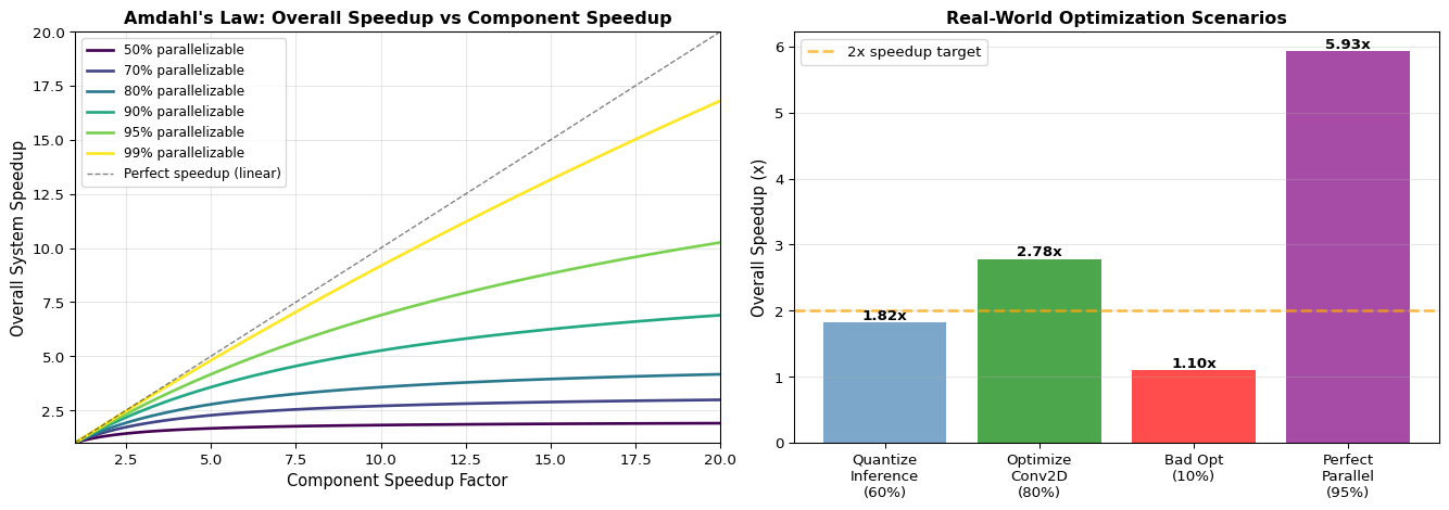
import numpy as npimport matplotlib.pyplot as pltdef amdahls_law(parallel_fraction, speedup_factor):""" Calculate theoretical speedup using Amdahl's Law Overall speedup = 1 / ((1 - P) + P/S) where P = fraction that can be parallelized/optimized S = speedup factor for that fraction """if parallel_fraction <0or parallel_fraction >1:raiseValueError("Parallel fraction must be between 0 and 1") serial_fraction =1- parallel_fraction speedup =1/ (serial_fraction + parallel_fraction / speedup_factor)return speedup# Example scenariosprint("="*70)print("Amdahl's Law: Optimization Scenarios")print("="*70)scenarios = [ {'name': 'Quantize inference (60% of time in MatMul)','parallel_fraction': 0.60,'speedup_factor': 4.0, # Int8 vs Float32'description': '60% of inference time is matrix multiplication, 4x faster with Int8' }, {'name': 'Optimize convolution (80% of time in Conv2D)','parallel_fraction': 0.80,'speedup_factor': 5.0, # CMSIS-NN optimization'description': '80% of inference time in Conv2D, 5x faster with CMSIS-NN' }, {'name': 'Bad optimization (only 10% of bottleneck)','parallel_fraction': 0.10,'speedup_factor': 10.0, # 10x faster but small fraction'description': 'Optimized part is 10x faster but only 10% of total time' }, {'name': 'Perfect parallelization (95% parallelizable)','parallel_fraction': 0.95,'speedup_factor': 8.0, # 8 cores'description': '95% can be parallelized across 8 cores' }]for scenario in scenarios: speedup = amdahls_law(scenario['parallel_fraction'], scenario['speedup_factor'])print(f"\n{scenario['name']}:")print(f" {scenario['description']}")print(f" Parallel fraction: {scenario['parallel_fraction']*100:.0f}%")print(f" Component speedup: {scenario['speedup_factor']:.1f}x")print(f" Overall speedup: {speedup:.2f}x")print(f" Time reduction: {(1-1/speedup)*100:.1f}%")# Visualize Amdahl's Law for different parallel fractionsfig, (ax1, ax2) = plt.subplots(1, 2, figsize=(14, 5))# Plot 1: Speedup vs component speedup for different parallel fractionsspeedup_factors = np.linspace(1, 20, 100)parallel_fractions = [0.5, 0.7, 0.8, 0.9, 0.95, 0.99]colors = plt.cm.viridis(np.linspace(0, 1, len(parallel_fractions)))for pf, color inzip(parallel_fractions, colors): speedups = [amdahls_law(pf, sf) for sf in speedup_factors] ax1.plot(speedup_factors, speedups, label=f'{pf*100:.0f}% parallelizable', linewidth=2, color=color)ax1.plot(speedup_factors, speedup_factors, 'k--', linewidth=1, label='Perfect speedup (linear)', alpha=0.5)ax1.set_xlabel('Component Speedup Factor', fontsize=11)ax1.set_ylabel('Overall System Speedup', fontsize=11)ax1.set_title("Amdahl's Law: Overall Speedup vs Component Speedup", fontweight='bold')ax1.legend(loc='upper left', fontsize=9)ax1.grid(True, alpha=0.3)ax1.set_xlim(1, 20)ax1.set_ylim(1, 20)# Plot 2: Practical optimization examplesopt_names = ['Quantize\nInference\n(60%)', 'Optimize\nConv2D\n(80%)','Bad Opt\n(10%)', 'Perfect\nParallel\n(95%)']opt_speedups = [ amdahls_law(0.60, 4.0), amdahls_law(0.80, 5.0), amdahls_law(0.10, 10.0), amdahls_law(0.95, 8.0)]bars = ax2.bar(opt_names, opt_speedups, color=['steelblue', 'green', 'red', 'purple'], alpha=0.7)ax2.axhline(y=2, color='orange', linestyle='--', linewidth=2, label='2x speedup target', alpha=0.7)ax2.set_ylabel('Overall Speedup (x)', fontsize=11)ax2.set_title('Real-World Optimization Scenarios', fontweight='bold')ax2.legend()ax2.grid(True, alpha=0.3, axis='y')# Add value labels on barsfor bar in bars: height = bar.get_height() ax2.text(bar.get_x() + bar.get_width()/2., height,f'{height:.2f}x', ha='center', va='bottom', fontsize=10, fontweight='bold')plt.tight_layout()plt.show()# Key insightprint("\n"+"="*70)print("Key Insight:")print("="*70)print("Optimizing a small fraction of code yields limited overall speedup,")print("even with massive component speedup. Always profile to find the")print("actual bottleneck before optimizing!")
======================================================================
Amdahl's Law: Optimization Scenarios
======================================================================

Quantize inference (60% of time in MatMul):
  60% of inference time is matrix multiplication, 4x faster with Int8
  Parallel fraction: 60%
  Component speedup: 4.0x
  Overall speedup:   1.82x
  Time reduction:    45.0%

Optimize convolution (80% of time in Conv2D):
  80% of inference time in Conv2D, 5x faster with CMSIS-NN
  Parallel fraction: 80%
  Component speedup: 5.0x
  Overall speedup:   2.78x
  Time reduction:    64.0%

Bad optimization (only 10% of bottleneck):
  Optimized part is 10x faster but only 10% of total time
  Parallel fraction: 10%
  Component speedup: 10.0x
  Overall speedup:   1.10x
  Time reduction:    9.0%

Perfect parallelization (95% parallelizable):
  95% can be parallelized across 8 cores
  Parallel fraction: 95%
  Component speedup: 8.0x
  Overall speedup:   5.93x
  Time reduction:    83.1%

======================================================================
Key Insight:
======================================================================
Optimizing a small fraction of code yields limited overall speedup,
even with massive component speedup. Always profile to find the
actual bottleneck before optimizing!
Interactive Notebook
The notebook below contains runnable code for all Level 1 activities.
LAB 11: Edge Device Profiling and Performance Analysis
Apply the roofline model - Identify compute vs memory-bound operations
Measure real-world inference metrics - Latency, throughput, energy estimation
Prerequisites Check
Before You Begin
Make sure you have completed: - [ ] LAB 02: ML Foundations with TensorFlow - [ ] LAB 03: Model Quantization - [ ] Understanding of neural network layer types
Part 1: Computational Complexity Theory
1.1 Why Profiling Matters for Edge
Edge devices have strict constraints that differ from cloud/desktop:
Environment: local Jupyter or Colab, no hardware required.
Use this level to build intuition before touching devices. Suggested workflow:
Load one or more models from earlier labs (e.g., LAB03 quantized classifier, LAB04 keyword spotter, LAB10 EMG classifier).
Inspect the model architecture and parameter count (model.summary()).
Estimate model file size and tensor arena needs (Float32 vs Int8).
Run microbenchmarks on your laptop (or a Raspberry Pi) to estimate relative latency.
Record a short table in your notes for each model: parameters, on-disk size, and estimated MCU latency.
Then reflect: which model(s) look viable for Arduino Nano 33 BLE / ESP32 given their RAM/Flash limits?
Here we “simulate” deployment by running real firmware on a development board and using serial output for profiling. You do not need a power sensor yet.
Suggested steps (Arduino Nano 33 BLE / ESP32):
Take a working TFLite Micro sketch from LAB05, LAB04 (KWS), or LAB10 (EMG).
Add timing code using micros() around the inference call, and print per‑inference latency.
Enable and log any available memory reports (e.g., ESP.getFreeHeap() on ESP32 or custom freeMemory() on AVR).
Run a statistical benchmark:
Ignore the first few “warm-up” inferences.
Collect 50–100 measurements.
Compute mean, min/max, and standard deviation (either on-device or by copying logs into the notebook).
Plot latency histograms / time series in the notebook and identify:
Typical latency vs worst-case latency
Any abnormal spikes (e.g., due to WiFi, interrupts, GC)
Outcome: a clear picture of latency and memory behaviour for at least one model on a real board, without yet worrying about power.
Now add hardware power measurement using an INA219 current sensor or a USB power meter.
Wire the INA219 in series with your target board’s supply (as in Chapter 11 diagrams).
Use a separate Arduino or your dev board to read INA219 voltage/current and stream logs over Serial.
Run three profiling phases:
Idle loop (no work)
CPU‑bound benchmark (e.g., sin() loop from the chapter)
ML inference workload (e.g., KWS or EMG model)
Capture logs into a CSV file and compute:
Average current and power in each phase
Energy per inference for the ML workload
Estimated battery life for a given battery capacity and duty cycle
Summarise your findings in a short report:
Where is the energy going (idle, compute, radio)?
Are there easy wins (sleep modes, batching, quantization) that meaningfully change battery life?
If you do not have an INA219, you can still complete the lab conceptually using:
A USB power meter (less detailed, but still useful).
Typical current figures from datasheets plus your measured duty cycles to estimate energy.
Visual Troubleshooting
Real-Time Performance Issues
flowchart TD
    A[Inference too slow] --> B{Platform?}
    B -->|Microcontroller| C{Model size?}
    C -->|Large| D[Reduce complexity:<br/>Fewer layers<br/>Smaller kernels 3x3<br/>Reduce channels<br/>Depthwise separable conv]
    C -->|Minimal| E[Optimize ops:<br/>CMSIS-NN acceleration<br/>Check optimized kernels<br/>Profile bottleneck layers]
    B -->|Raspberry Pi| F{Using TFLite?}
    F -->|Full TensorFlow| G[Switch to TFLite:<br/>4-10x faster<br/>interpreter = tf.lite.Interpreter]
    F -->|TFLite| H[Enable threading:<br/>num_threads=4<br/>Use all CPU cores]

    style A fill:#ff6b6b
    style D fill:#4ecdc4
    style E fill:#4ecdc4
    style G fill:#4ecdc4
    style H fill:#4ecdc4
---title: "LAB11: Profiling and Optimization"subtitle: "Performance Analysis for Edge Devices"---::: {.callout-note}## PDF Textbook ReferenceFor detailed theoretical foundations, mathematical proofs, and algorithm derivations, see **Chapter 11: Edge Device Profiling and Optimization** in the [PDF textbook](../downloads/Edge-Analytics-Lab-Book-v1.0.0.pdf).The PDF chapter includes:- Detailed timing measurement theory and timer resolution analysis- Complete memory profiling methodology and tools- In-depth power measurement circuits and INA219 theory- Mathematical models for performance bottleneck identification- Comprehensive optimization strategies with theoretical justifications:::[](https://colab.research.google.com/github/ngcharithperera/edge-analytics-lab-book/blob/main/notebooks/LAB11_profiling.ipynb)[Download Notebook](https://raw.githubusercontent.com/ngcharithperera/edge-analytics-lab-book/main/notebooks/LAB11_profiling.ipynb)## Learning ObjectivesBy the end of this lab you should be able to:- Measure code execution time on microcontrollers using millisecond and microsecond timers- Profile memory footprint (SRAM/Flash/tensor arena) of TinyML applications- Measure power consumption and estimate battery life for typical workloads- Compare Float32 vs Int8 models in terms of size, latency, and accuracy- Apply targeted optimizations based on profiling results rather than guesswork## Theory SummaryProfiling transforms speculation into science. Edge devices have severe constraints—Arduino Nano 33 BLE offers 256 KB SRAM and runs at 64 MHz, compared to laptops with 16 GB RAM and 3+ GHz CPUs (a 60,000x memory gap and 50x speed gap). Without measurement, you cannot know if your ML model will fit, run fast enough for real-time requirements, or drain the battery in hours versus months.**Timing measurement** uses `millis()` (1 ms resolution) for operations >10 ms and `micros()` (4 μs resolution on most boards) for fast operations. Critical insight: **always discard the first run** as warmup to eliminate cache-loading effects that can inflate latency 2-10x. Statistical benchmarking runs 50-100 trials to compute mean, standard deviation, min/max, and percentiles (p95, p99). High variance indicates inconsistent execution—often from interrupts, dynamic memory allocation, or unstable power supply.**Memory profiling** distinguishes three regions: (1) **Flash** stores compiled code and model weights (persistent, abundant at 1-4 MB), (2) **SRAM** holds variables, stack, heap, and TensorFlow's tensor arena (volatile, scarce at 8-256 KB), (3) **Tensor arena** is the critical bottleneck—TensorFlow Lite Micro allocates this contiguous block for activation tensors during inference. Int8 quantization typically reduces both model size and arena requirements by 3-4x compared to Float32. The ESP32's `getMinFreeHeap()` reveals peak memory usage—if this approaches zero, your application will crash unpredictably.**Power profiling** uses INA219 current sensors or USB power meters to measure actual consumption. Key principle: **average current determines battery life**. For duty-cycled operation (wake periodically, run inference, sleep), compute weighted average: (I_active × t_active + I_sleep × t_sleep) / (t_active + t_sleep). Example: ESP32 deep sleep at 0.01 mA, active inference at 80 mA for 2 seconds per minute yields 2.68 mA average → 2000 mAh battery lasts 750 hours (31 days) versus 25 hours if continuously active. Optimization often targets duty cycling over raw inference speed.::: {.callout-tip}## Key Concepts at a Glance- **Timing Functions**: `millis()` for ms resolution (ops >10 ms), `micros()` for μs resolution (fast ops); both use unsigned long to handle overflow at 49 days / 71 minutes- **Statistical Benchmarking**: Discard first 1-5 runs (warmup), collect 50-100 samples, report mean ± std, min/max, p95/p99; high variance indicates instability- **Memory Hierarchy**: Flash (code + model weights, 1-4 MB), SRAM (variables + stack + heap + tensor arena, 8-256 KB), Tensor Arena (TFLite working memory, 2-30 KB typical)- **Compile-Time vs Runtime**: Arduino IDE reports global variable usage (~15% SRAM for "hello world") but misses dynamic allocations; runtime profiling via `ESP.getFreeHeap()` or `freeMemory()` shows actual usage- **Int8 vs Float32**: Quantization yields 3-4x model size reduction, 2.5-3x arena reduction, 3-5x speed improvement, <1% accuracy loss for most models- **Power Measurement**: INA219 sensor measures voltage and current via I2C; calculate energy/inference = V × I × t; estimate battery life = capacity / average_current- **Optimization Decision Tree**: Profile first → identify bottleneck (memory/latency/power) → apply targeted fix → profile again to verify; don't optimize blindly!:::::: {.callout-warning}## Common Pitfalls1. **Reporting first-run latency**: The initial inference is 2-10x slower due to cache warmup and lazy initialization. Always run 5+ warmup iterations before collecting timing data, or clearly label cold-start vs warm latency.2. **Ignoring standard deviation**: Reporting only mean latency hides critical variance. A system with 50 ms ± 30 ms cannot meet a 60 ms deadline (p99 > 100 ms). Real-time systems care about worst-case (max or p99), not average.3. **Confusing compile-time and runtime memory**: Arduino IDE reports 15% SRAM used, but runtime crashes when allocating tensor arena. Compile-time only counts global variables; dynamic allocations (stack growth, heap fragmentation) appear at runtime.4. **Insufficient power supply for measurement**: USB ports provide 500 mA, but WiFi bursts draw 240 mA. Voltage sag causes clock jitter and timing measurement errors. Use stable 1A+ supply for accurate profiling.5. **Optimizing the wrong bottleneck**: Speeding up inference 2x doesn't help if deep sleep dominates battery life. Profile to find actual bottleneck: 60% time in memory allocation → fix memory, not computation. Measure before optimizing!:::## Quick Reference### Key Formulas**Battery Life with Duty Cycling**$$I_{\text{avg}} = \frac{I_{\text{active}} \cdot t_{\text{active}} + I_{\text{sleep}} \cdot t_{\text{sleep}}}{t_{\text{active}} + t_{\text{sleep}}}$$$$\text{Battery Life (hours)} = \frac{\text{Capacity (mAh)}}{I_{\text{avg}} \text{ (mA)}}$$**Energy Per Inference**$$E_{\text{inference}} = V \times I_{\text{active}} \times t_{\text{inference}} \quad \text{(in Joules or mJ)}$$**Memory Requirements Estimation**$$\text{Model Size (bytes)} \approx \text{Parameters} \times \begin{cases}4 & \text{Float32} \\ 1 & \text{Int8}\end{cases}$$$$\text{Tensor Arena (bytes)} \approx 2-3 \times \text{Model Size} \quad \text{(heuristic)}$$**Speedup Factor from Quantization**$$\text{Speedup} = \frac{t_{\text{Float32}}}{t_{\text{Int8}}} \approx 3-5\times \quad \text{(typical range)}$$### Important Parameter Values| **Metric** | **Device** | **Typical Value** | **Range** | **Notes** ||------------|------------|-------------------|-----------|-----------|| **Timing Resolution** | Arduino Uno | 4 μs | 4-16 μs | `micros()` resolution || | ESP32 | 1 μs | 1 μs | Better precision || **Memory (SRAM)** | Arduino Uno | 2 KB | - | Very constrained || | Nano 33 BLE | 256 KB | - | Fits small models || | ESP32 | 520 KB | - | Fits medium models || **Flash** | Arduino Uno | 32 KB | - | Code + model storage || | Nano 33 BLE | 1 MB | - | Plenty for models || | ESP32 | 4 MB | - | Large model support || **Power (Active)** | Nano 33 BLE | 15-25 mA | 5-80 mA | Depends on workload || | ESP32 (CPU) | 80 mA | 20-240 mA | WiFi adds 160+ mA || **Power (Sleep)** | Nano 33 BLE | - | - | No native deep sleep || | ESP32 (deep) | 10 μA | 5-150 μA | Best-in-class || **Inference Latency** | Tiny MLP (Int8) | 1-2 ms | 0.5-5 ms | 784→32→10 on Nano || | Small CNN (Int8) | 10-20 ms | 5-40 ms | Keyword spotting || | MobileNet (Int8) | 800+ ms | 500-1500 ms | Person detection |### Essential Code Patterns**Statistical Timing Benchmark**```cpp#define NUM_TRIALS 100unsignedlong times[NUM_TRIALS];void benchmark(){// Warmup runInference();// Measurefor(int i =0; i < NUM_TRIALS; i++){unsignedlong start = micros(); runInference(); times[i]= micros()- start;}// Statisticsfloat mean =0;for(int i =0; i < NUM_TRIALS; i++) mean += times[i]; mean /= NUM_TRIALS; Serial.print("Mean: "); Serial.print(mean/1000,2); Serial.println(" ms");}```**Free Memory Check (ESP32)**```cppvoid checkMemory(){ Serial.print("Free heap: "); Serial.print(ESP.getFreeHeap()); Serial.println(" bytes"); Serial.print("Min free heap: "); Serial.print(ESP.getMinFreeHeap()); Serial.println(" bytes");}```**Power Measurement with INA219**```cpp#include <Adafruit_INA219.h>Adafruit_INA219 ina219;void measurePower(){float voltage = ina219.getBusVoltage_V();float current = ina219.getCurrent_mA();float power = ina219.getPower_mW(); Serial.print(voltage,3); Serial.print(","); Serial.print(current,2); Serial.print(","); Serial.println(power,2);}```### PDF Cross-References- **Section 2**: Timing measurement with millis() and micros() (pages 3-6)- **Section 3**: Memory profiling techniques (pages 7-12)- **Section 4**: Power consumption measurement with INA219 (pages 13-17)- **Section 6**: TFLite Micro inference profiling (pages 21-25)- **Section 7**: Float32 vs Int8 quantization comparison (pages 26-28)- **Section 8**: Complete profiling workflow example (pages 29-33)- **Section 10**: Case studies showing optimization decisions (pages 36-40)## Self-Assessment CheckpointsTest your understanding before proceeding to the exercises.::: {.callout-note collapse="true" title="Question 1: Your model's first inference takes 180ms but subsequent inferences take 45ms. Why the difference?"}**Answer:** Cold start vs warm execution. The first inference includes: (1) **Cache warming** - loading model weights from Flash into CPU cache, (2) **Lazy initialization** - TensorFlow Lite Micro initializes operations on first use, (3) **Memory allocation** - tensor arena setup and alignment. Subsequent inferences benefit from cached weights and initialized operators. Always discard the first 1-5 runs when benchmarking and report: "Cold start: 180ms, Warm: 45ms ± 3ms (N=100 runs)". Real-time systems care about both - cold start affects wake-from-sleep latency, warm latency affects continuous operation.:::::: {.callout-note collapse="true" title="Question 2: Arduino IDE reports '15% SRAM used' but your program crashes with out-of-memory. Explain why."}**Answer:** Compile-time vs runtime memory. The IDE's 15% only counts **global/static variables** visible to the linker. It misses: (1) **Stack growth** from function calls and local variables (8-20KB typical), (2) **Heap allocations** including tensor arena (30-100KB for ML models), (3) **Runtime buffers** for sensors, communication, and processing. A program showing 15% static usage might actually need 80% SRAM at runtime. Solutions: Use `ESP.getFreeHeap()` or `freeMemory()` during execution to measure actual usage, declare tensor arena static with known size, minimize dynamic allocations, and always leave 20%+ headroom for stack growth.:::::: {.callout-note collapse="true" title="Question 3: Calculate the memory savings from quantizing a 100,000-parameter model from float32 to int8."}**Answer:** Model size reduction: Float32 = 100,000 params × 4 bytes = 400,000 bytes = 400 KB. Int8 = 100,000 params × 1 byte = 100,000 bytes = 100 KB. Savings = 400 - 100 = 300 KB (75% reduction). Tensor arena reduction (typical): Float32 arena ≈ 800 KB (2× model size). Int8 arena ≈ 250 KB (2.5× model size). Total SRAM savings ≈ 550 KB. This is the difference between "won't fit on Arduino Nano 33 BLE (256KB SRAM)" and "fits comfortably with room for sensors and buffers.":::::: {.callout-note collapse="true" title="Question 4: Your inference latency shows: mean=50ms, std=25ms, max=180ms. Is this acceptable for real-time gesture recognition requiring <100ms response?"}**Answer:** No, this is unacceptable. While the mean (50ms) looks good, the high standard deviation (±25ms) and especially the max (180ms) violate the <100ms requirement. For real-time systems, **worst-case latency** matters more than average. With 25ms std, approximately 5% of inferences exceed 100ms (mean + 2σ = 100ms). Better metric: report p95 or p99 percentiles. Solutions: (1) Investigate max latency causes (interrupts, garbage collection, cache misses), (2) Reduce model complexity if computational bottleneck, (3) Use priority scheduling to prevent interrupt interference, (4) Set hard deadline with watchdog timer. Aim for: "p99 < 80ms" to ensure <100ms with margin.:::::: {.callout-note collapse="true" title="Question 5: Your profiling shows 60% of inference time is spent in memory allocation. Should you optimize the ML model operations or fix memory management first?"}**Answer:** Fix memory management first! Profiling reveals the actual bottleneck. If 60% of time is memory allocation, speeding up convolution ops by 2× only improves total time by ~15% (40% of time × 2× faster = 20% reduction). Instead: (1) **Pre-allocate buffers** - declare static arrays instead of malloc/free each inference, (2) **Reduce allocations** - reuse buffers for intermediate results, (3) **Fix tensor arena size** - start with adequate size to avoid reallocation. After fixing memory (now 10% of time instead of 60%), THEN optimize model ops if needed. This is why profiling matters: guessing leads to optimizing the wrong thing. Always profile → identify bottleneck → fix bottleneck → profile again → repeat.:::## Try It YourselfThese interactive Python examples demonstrate profiling and optimization concepts. Run them to understand performance analysis before implementing on embedded hardware.### FLOPs and Memory Estimation CalculatorEstimate computational requirements for neural networks:```{python}import numpy as npimport pandas as pddef calculate_flops_dense(input_size, output_size):"""Calculate FLOPs for a dense (fully connected) layer"""# Matrix multiply: input_size * output_size multiplications + additions# Plus bias addition: output_size additions multiply_adds = input_size * output_size bias_adds = output_size total_ops = multiply_adds *2+ bias_adds # Each MAC = 2 FLOPsreturn total_opsdef calculate_flops_conv2d(input_h, input_w, kernel_h, kernel_w, in_channels, out_channels, stride=1, padding=0):"""Calculate FLOPs for a 2D convolution layer"""# Output dimensions output_h = (input_h +2*padding - kernel_h) // stride +1 output_w = (input_w +2*padding - kernel_w) // stride +1# Operations per output position ops_per_output = kernel_h * kernel_w * in_channels *2# MACs = 2 FLOPs# Total operations total_ops = ops_per_output * output_h * output_w * out_channelsreturn total_opsdef calculate_memory(num_params, dtype='float32'):"""Calculate memory requirements for model parameters""" bytes_per_param = {'float32': 4, 'float16': 2, 'int8': 1, 'int16': 2}return num_params * bytes_per_param.get(dtype, 4)# Example: Tiny MLP for MNIST digit classificationprint("="*60)print("Example 1: Tiny MLP (784 -> 32 -> 10)")print("="*60)# Layer dimensionsinput_size =784# 28x28 flattenedhidden_size =32output_size =10# Calculate FLOPs per layerflops_layer1 = calculate_flops_dense(input_size, hidden_size)flops_relu = hidden_size # ReLU: 1 comparison per neuronflops_layer2 = calculate_flops_dense(hidden_size, output_size)total_flops = flops_layer1 + flops_relu + flops_layer2# Calculate parametersparams_layer1 = input_size * hidden_size + hidden_size # weights + biasesparams_layer2 = hidden_size * output_size + output_sizetotal_params = params_layer1 + params_layer2# Memory for different dtypesmemory_float32 = calculate_memory(total_params, 'float32')memory_int8 = calculate_memory(total_params, 'int8')print(f"\nLayer 1 (Dense 784->32):")print(f" Parameters: {params_layer1:,}")print(f" FLOPs: {flops_layer1:,}")print(f"\nLayer 2 (Dense 32->10):")print(f" Parameters: {params_layer2:,}")print(f" FLOPs: {flops_layer2:,}")print(f"\nTotal Model:")print(f" Parameters: {total_params:,}")print(f" FLOPs/inference: {total_flops:,}")print(f"\nMemory Requirements:")print(f" Float32: {memory_float32:,} bytes ({memory_float32/1024:.1f} KB)")print(f" Int8: {memory_int8:,} bytes ({memory_int8/1024:.1f} KB)")print(f" Savings: {(1- memory_int8/memory_float32)*100:.1f}%")# Example 2: Small CNN for keyword spottingprint("\n"+"="*60)print("Example 2: Small CNN (10x20 -> Conv -> Dense)")print("="*60)input_h, input_w =10, 20# 10 time frames, 20 frequency binskernel_h, kernel_w =3, 3in_channels =1out_channels =8stride =1padding =0# Conv layer FLOPsconv_flops = calculate_flops_conv2d(input_h, input_w, kernel_h, kernel_w, in_channels, out_channels, stride, padding)conv_params = kernel_h * kernel_w * in_channels * out_channels + out_channels# Output size after convoutput_h = (input_h +2*padding - kernel_h) // stride +1output_w = (input_w +2*padding - kernel_w) // stride +1flatten_size = output_h * output_w * out_channels# Dense layerdense_units =4# 4-class classificationdense_flops = calculate_flops_dense(flatten_size, dense_units)dense_params = flatten_size * dense_units + dense_unitstotal_params_cnn = conv_params + dense_paramstotal_flops_cnn = conv_flops + dense_flopsprint(f"\nConv2D Layer ({in_channels}@{input_h}x{input_w} -> {out_channels}@{output_h}x{output_w}):")print(f" Parameters: {conv_params:,}")print(f" FLOPs: {conv_flops:,}")print(f"\nDense Layer ({flatten_size} -> {dense_units}):")print(f" Parameters: {dense_params:,}")print(f" FLOPs: {dense_flops:,}")print(f"\nTotal CNN:")print(f" Parameters: {total_params_cnn:,}")print(f" FLOPs/inference: {total_flops_cnn:,}")print(f" Memory (Float32): {calculate_memory(total_params_cnn, 'float32'):,} bytes")print(f" Memory (Int8): {calculate_memory(total_params_cnn, 'int8'):,} bytes")# Create comparison tablemodels = [ {'Model': 'Tiny MLP', 'Params': total_params, 'FLOPs': total_flops,'Float32 (KB)': memory_float32/1024, 'Int8 (KB)': memory_int8/1024}, {'Model': 'Small CNN', 'Params': total_params_cnn, 'FLOPs': total_flops_cnn,'Float32 (KB)': calculate_memory(total_params_cnn, 'float32')/1024,'Int8 (KB)': calculate_memory(total_params_cnn, 'int8')/1024}]df = pd.DataFrame(models)print("\n"+"="*60)print("Model Comparison:")print("="*60)print(df.to_string(index=False))```### Tensor Arena Memory EstimationEstimate TensorFlow Lite Micro memory requirements:```{python}import numpy as npimport matplotlib.pyplot as pltdef estimate_tensor_arena(layer_configs, dtype='int8'):""" Estimate tensor arena size for a sequential model Arena needs to store intermediate activations for the largest layer(s) """ bytes_per_element = {'float32': 4, 'int8': 1} bytes_elem = bytes_per_element[dtype] max_activation_size =0 layer_sizes = []for i, layer inenumerate(layer_configs): layer_type = layer['type']if layer_type =='dense':# Dense layer stores input and output activations input_size = layer['input_size'] output_size = layer['output_size']# Need both input and output during computation activation_bytes = (input_size + output_size) * bytes_elem layer_sizes.append({'layer': f"Dense_{i}",'input': input_size,'output': output_size,'bytes': activation_bytes }) max_activation_size =max(max_activation_size, activation_bytes)elif layer_type =='conv2d':# Conv layer stores input and output feature maps input_h, input_w, input_c = layer['input_shape'] output_h, output_w, output_c = layer['output_shape'] input_bytes = input_h * input_w * input_c * bytes_elem output_bytes = output_h * output_w * output_c * bytes_elem activation_bytes = input_bytes + output_bytes layer_sizes.append({'layer': f"Conv2D_{i}",'input': input_h * input_w * input_c,'output': output_h * output_w * output_c,'bytes': activation_bytes }) max_activation_size =max(max_activation_size, activation_bytes)# Add overhead for TFLite interpreter (~2-3KB typical) overhead =2048# Rule of thumb: tensor arena ≈ 2-3x max activation size (for TFLite bookkeeping) estimated_arena =int(max_activation_size *2.5) + overheadreturn estimated_arena, layer_sizes# Example 1: Tiny MLPmlp_config = [ {'type': 'dense', 'input_size': 784, 'output_size': 32}, {'type': 'dense', 'input_size': 32, 'output_size': 10}]arena_mlp_float, layers_mlp_float = estimate_tensor_arena(mlp_config, dtype='float32')arena_mlp_int8, layers_mlp_int8 = estimate_tensor_arena(mlp_config, dtype='int8')print("="*60)print("Tensor Arena Estimation: Tiny MLP")print("="*60)print(f"\nFloat32:")print(f" Estimated arena: {arena_mlp_float:,} bytes ({arena_mlp_float/1024:.1f} KB)")print(f"\nInt8:")print(f" Estimated arena: {arena_mlp_int8:,} bytes ({arena_mlp_int8/1024:.1f} KB)")print(f"\nMemory savings: {(1- arena_mlp_int8/arena_mlp_float)*100:.1f}%")# Example 2: Small CNNcnn_config = [ {'type': 'conv2d', 'input_shape': (10, 20, 1), 'output_shape': (8, 18, 8)}, {'type': 'dense', 'input_size': 8*18*8, 'output_size': 4}]arena_cnn_float, layers_cnn_float = estimate_tensor_arena(cnn_config, dtype='float32')arena_cnn_int8, layers_cnn_int8 = estimate_tensor_arena(cnn_config, dtype='int8')print("\n"+"="*60)print("Tensor Arena Estimation: Small CNN")print("="*60)print(f"\nFloat32:")print(f" Estimated arena: {arena_cnn_float:,} bytes ({arena_cnn_float/1024:.1f} KB)")print(f"\nInt8:")print(f" Estimated arena: {arena_cnn_int8:,} bytes ({arena_cnn_int8/1024:.1f} KB)")print(f"\nMemory savings: {(1- arena_cnn_int8/arena_cnn_float)*100:.1f}%")# Visualize memory breakdownfig, (ax1, ax2) = plt.subplots(1, 2, figsize=(14, 5))# Memory comparisonmodels = ['Tiny MLP', 'Small CNN']float32_sizes = [arena_mlp_float/1024, arena_cnn_float/1024]int8_sizes = [arena_mlp_int8/1024, arena_cnn_int8/1024]x = np.arange(len(models))width =0.35bars1 = ax1.bar(x - width/2, float32_sizes, width, label='Float32', color='steelblue')bars2 = ax1.bar(x + width/2, int8_sizes, width, label='Int8', color='darkorange')ax1.set_ylabel('Tensor Arena Size (KB)')ax1.set_title('Memory Requirements by Model and Data Type', fontweight='bold')ax1.set_xticks(x)ax1.set_xticklabels(models)ax1.legend()ax1.grid(True, alpha=0.3, axis='y')# Add value labels on barsfor bars in [bars1, bars2]:for bar in bars: height = bar.get_height() ax1.text(bar.get_x() + bar.get_width()/2., height,f'{height:.1f} KB', ha='center', va='bottom', fontsize=9)# Device capacity comparisondevices = ['Arduino Uno\n(2 KB)', 'Nano 33 BLE\n(256 KB)', 'ESP32\n(520 KB)']capacities = [2, 256, 520]colors_fit = ['red', 'green', 'green']bars = ax2.barh(devices, capacities, color=colors_fit, alpha=0.6)ax2.axvline(x=arena_mlp_int8/1024, color='orange', linestyle='--', linewidth=2, label=f'Tiny MLP Int8 ({arena_mlp_int8/1024:.1f} KB)')ax2.axvline(x=arena_cnn_int8/1024, color='purple', linestyle='--', linewidth=2, label=f'Small CNN Int8 ({arena_cnn_int8/1024:.1f} KB)')ax2.set_xlabel('SRAM Capacity (KB)')ax2.set_title('Device Memory Capacity vs Model Requirements', fontweight='bold')ax2.legend()ax2.grid(True, alpha=0.3, axis='x')ax2.set_xlim(0, 550)plt.tight_layout()plt.show()# Feasibility checkprint("\n"+"="*60)print("Device Feasibility Analysis:")print("="*60)for device, capacity in [('Arduino Uno', 2*1024), ('Nano 33 BLE', 256*1024), ('ESP32', 520*1024)]: mlp_fit ="YES"if arena_mlp_int8 < capacity *0.7else"NO" cnn_fit ="YES"if arena_cnn_int8 < capacity *0.7else"NO"print(f"\n{device} ({capacity/1024:.0f} KB SRAM):")print(f" Tiny MLP (Int8): {mlp_fit}")print(f" Small CNN (Int8): {cnn_fit}")```### Amdahl's Law Speedup CalculatorCalculate theoretical speedup from optimization:```{python}import numpy as npimport matplotlib.pyplot as pltdef amdahls_law(parallel_fraction, speedup_factor):""" Calculate theoretical speedup using Amdahl's Law Overall speedup = 1 / ((1 - P) + P/S) where P = fraction that can be parallelized/optimized S = speedup factor for that fraction """if parallel_fraction <0or parallel_fraction >1:raiseValueError("Parallel fraction must be between 0 and 1") serial_fraction =1- parallel_fraction speedup =1/ (serial_fraction + parallel_fraction / speedup_factor)return speedup# Example scenariosprint("="*70)print("Amdahl's Law: Optimization Scenarios")print("="*70)scenarios = [ {'name': 'Quantize inference (60% of time in MatMul)','parallel_fraction': 0.60,'speedup_factor': 4.0, # Int8 vs Float32'description': '60% of inference time is matrix multiplication, 4x faster with Int8' }, {'name': 'Optimize convolution (80% of time in Conv2D)','parallel_fraction': 0.80,'speedup_factor': 5.0, # CMSIS-NN optimization'description': '80% of inference time in Conv2D, 5x faster with CMSIS-NN' }, {'name': 'Bad optimization (only 10% of bottleneck)','parallel_fraction': 0.10,'speedup_factor': 10.0, # 10x faster but small fraction'description': 'Optimized part is 10x faster but only 10% of total time' }, {'name': 'Perfect parallelization (95% parallelizable)','parallel_fraction': 0.95,'speedup_factor': 8.0, # 8 cores'description': '95% can be parallelized across 8 cores' }]for scenario in scenarios: speedup = amdahls_law(scenario['parallel_fraction'], scenario['speedup_factor'])print(f"\n{scenario['name']}:")print(f" {scenario['description']}")print(f" Parallel fraction: {scenario['parallel_fraction']*100:.0f}%")print(f" Component speedup: {scenario['speedup_factor']:.1f}x")print(f" Overall speedup: {speedup:.2f}x")print(f" Time reduction: {(1-1/speedup)*100:.1f}%")# Visualize Amdahl's Law for different parallel fractionsfig, (ax1, ax2) = plt.subplots(1, 2, figsize=(14, 5))# Plot 1: Speedup vs component speedup for different parallel fractionsspeedup_factors = np.linspace(1, 20, 100)parallel_fractions = [0.5, 0.7, 0.8, 0.9, 0.95, 0.99]colors = plt.cm.viridis(np.linspace(0, 1, len(parallel_fractions)))for pf, color inzip(parallel_fractions, colors): speedups = [amdahls_law(pf, sf) for sf in speedup_factors] ax1.plot(speedup_factors, speedups, label=f'{pf*100:.0f}% parallelizable', linewidth=2, color=color)ax1.plot(speedup_factors, speedup_factors, 'k--', linewidth=1, label='Perfect speedup (linear)', alpha=0.5)ax1.set_xlabel('Component Speedup Factor', fontsize=11)ax1.set_ylabel('Overall System Speedup', fontsize=11)ax1.set_title("Amdahl's Law: Overall Speedup vs Component Speedup", fontweight='bold')ax1.legend(loc='upper left', fontsize=9)ax1.grid(True, alpha=0.3)ax1.set_xlim(1, 20)ax1.set_ylim(1, 20)# Plot 2: Practical optimization examplesopt_names = ['Quantize\nInference\n(60%)', 'Optimize\nConv2D\n(80%)','Bad Opt\n(10%)', 'Perfect\nParallel\n(95%)']opt_speedups = [ amdahls_law(0.60, 4.0), amdahls_law(0.80, 5.0), amdahls_law(0.10, 10.0), amdahls_law(0.95, 8.0)]bars = ax2.bar(opt_names, opt_speedups, color=['steelblue', 'green', 'red', 'purple'], alpha=0.7)ax2.axhline(y=2, color='orange', linestyle='--', linewidth=2, label='2x speedup target', alpha=0.7)ax2.set_ylabel('Overall Speedup (x)', fontsize=11)ax2.set_title('Real-World Optimization Scenarios', fontweight='bold')ax2.legend()ax2.grid(True, alpha=0.3, axis='y')# Add value labels on barsfor bar in bars: height = bar.get_height() ax2.text(bar.get_x() + bar.get_width()/2., height,f'{height:.2f}x', ha='center', va='bottom', fontsize=10, fontweight='bold')plt.tight_layout()plt.show()# Key insightprint("\n"+"="*70)print("Key Insight:")print("="*70)print("Optimizing a small fraction of code yields limited overall speedup,")print("even with massive component speedup. Always profile to find the")print("actual bottleneck before optimizing!")```## Interactive NotebookThe notebook below contains runnable code for all Level 1 activities.{{< embed ../../notebooks/LAB11_profiling.ipynb >}}## Three-Tier Activities::: {.panel-tabset}### Level 1: NotebookEnvironment: local Jupyter or Colab, no hardware required.Use this level to build intuition before touching devices. Suggested workflow:1. Load one or more models from earlier labs (e.g., LAB03 quantized classifier, LAB04 keyword spotter, LAB10 EMG classifier).2. Inspect the model architecture and parameter count (`model.summary()`).3. Estimate model file size and tensor arena needs (Float32 vs Int8).4. Run microbenchmarks on your laptop (or a Raspberry Pi) to estimate relative latency.5. Record a short table in your notes for each model: parameters, on-disk size, and estimated MCU latency.Then reflect: which model(s) look viable for Arduino Nano 33 BLE / ESP32 given their RAM/Flash limits?### Level 2: SimulatorHere we “simulate” deployment by running real firmware on a development board and using serial output for profiling. You do **not** need a power sensor yet.Suggested steps (Arduino Nano 33 BLE / ESP32):1. Take a working TFLite Micro sketch from LAB05, LAB04 (KWS), or LAB10 (EMG).2. Add timing code using `micros()` around the inference call, and print per‑inference latency.3. Enable and log any available memory reports (e.g., `ESP.getFreeHeap()` on ESP32 or custom `freeMemory()` on AVR).4. Run a statistical benchmark: - Ignore the first few “warm-up” inferences. - Collect 50–100 measurements. - Compute mean, min/max, and standard deviation (either on-device or by copying logs into the notebook).5. Plot latency histograms / time series in the notebook and identify: - Typical latency vs worst-case latency - Any abnormal spikes (e.g., due to WiFi, interrupts, GC)Outcome: a clear picture of latency and memory behaviour for at least one model on a real board, **without** yet worrying about power.### Level 3: DeviceNow add hardware power measurement using an INA219 current sensor or a USB power meter.1. Wire the INA219 in series with your target board’s supply (as in Chapter 11 diagrams).2. Use a separate Arduino or your dev board to read INA219 voltage/current and stream logs over Serial.3. Run three profiling phases: - Idle loop (no work) - CPU‑bound benchmark (e.g., `sin()` loop from the chapter) - ML inference workload (e.g., KWS or EMG model)4. Capture logs into a CSV file and compute: - Average current and power in each phase - Energy per inference for the ML workload - Estimated battery life for a given battery capacity and duty cycle5. Summarise your findings in a short report: - Where is the energy going (idle, compute, radio)? - Are there easy wins (sleep modes, batching, quantization) that meaningfully change battery life?If you do not have an INA219, you can still complete the lab conceptually using:- A USB power meter (less detailed, but still useful).- Typical current figures from datasheets plus your measured duty cycles to estimate energy.:::## Visual Troubleshooting### Real-Time Performance Issues```{mermaid}flowchart TD A[Inference too slow] --> B{Platform?} B -->|Microcontroller| C{Model size?} C -->|Large| D[Reduce complexity:<br/>Fewer layers<br/>Smaller kernels 3x3<br/>Reduce channels<br/>Depthwise separable conv] C -->|Minimal| E[Optimize ops:<br/>CMSIS-NN acceleration<br/>Check optimized kernels<br/>Profile bottleneck layers] B -->|Raspberry Pi| F{Using TFLite?} F -->|Full TensorFlow| G[Switch to TFLite:<br/>4-10x faster<br/>interpreter = tf.lite.Interpreter] F -->|TFLite| H[Enable threading:<br/>num_threads=4<br/>Use all CPU cores] style A fill:#ff6b6b style D fill:#4ecdc4 style E fill:#4ecdc4 style G fill:#4ecdc4 style H fill:#4ecdc4```For complete troubleshooting flowcharts, see:- [Real-Time Performance Issues](../troubleshooting/index.qmd#real-time-performance-issues)- [Power Consumption Too High](../troubleshooting/index.qmd#power-consumption-too-high)- [All Visual Troubleshooting Guides](../troubleshooting/index.qmd)## Related Labs::: {.callout-tip}## Performance & Optimization- **LAB03: Quantization** - Model optimization before profiling- **LAB05: Edge Deployment** - Deploy models to profile on devices- **LAB15: Energy Optimization** - Advanced power optimization techniques:::::: {.callout-tip}## Apply Profiling To- **LAB04: Keyword Spotting** - Profile audio ML models- **LAB07: CNNs & Vision** - Profile vision models- **LAB10: EMG Biomedical** - Profile signal processing workloads:::## Related Resources- [Hardware Guide](../resources/hardware.qmd) - Equipment needed for Level 3- [Troubleshooting](../resources/troubleshooting.qmd) - Common issues and solutions