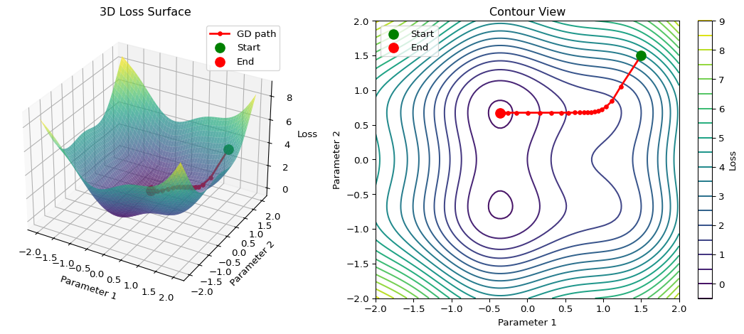
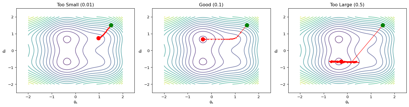
--- title: "Gradient Descent Visualizer" subtitle: "LAB02: Machine Learning Foundations" format: html: code-fold: true --- ## Interactive 3D Loss Surface ## Concept from LAB02 [ PDF book ](../downloads/Edge-Analytics-Lab-Book-v1.0.0.pdf) for the mathematical foundations.## The Visualization ```{python} #| label: fig-gradient-descent #| fig-cap: "Gradient descent on a 2D loss surface" #| code-fold: true import numpy as npimport matplotlib.pyplot as pltfrom mpl_toolkits.mplot3d import Axes3D# Create loss surface def loss_function(x, y):return x** 2 + y** 2 + 0.5 * np.sin(3 * x) + 0.5 * np.cos(3 * y)# Generate surface data = np.linspace(- 2 , 2 , 100 )= np.linspace(- 2 , 2 , 100 )= np.meshgrid(x, y)= loss_function(X, Y)# Gradient descent path def gradient(x, y):= 2 * x + 1.5 * np.cos(3 * x)= 2 * y - 1.5 * np.sin(3 * y)return dx, dy# Run gradient descent = [1.5 ], [1.5 ], [loss_function(1.5 , 1.5 )]= 0.1 for _ in range (50 ):= gradient(path_x[- 1 ], path_y[- 1 ])= path_x[- 1 ] - lr * dx= path_y[- 1 ] - lr * dy# Create figure = plt.figure(figsize= (12 , 5 ))# 3D surface plot = fig.add_subplot(121 , projection= '3d' )= 'viridis' , alpha= 0.7 , edgecolor= 'none' )'r.-' , linewidth= 2 , markersize= 8 , label= 'GD path' )0 ]], [path_y[0 ]], [path_z[0 ]], color= 'green' , s= 100 , label= 'Start' )- 1 ]], [path_y[- 1 ]], [path_z[- 1 ]], color= 'red' , s= 100 , label= 'End' )'Parameter 1' )'Parameter 2' )'Loss' )'3D Loss Surface' )# Contour plot = fig.add_subplot(122 )= ax2.contour(X, Y, Z, levels= 20 , cmap= 'viridis' )'r.-' , linewidth= 2 , markersize= 8 )0 ]], [path_y[0 ]], color= 'green' , s= 100 , zorder= 5 , label= 'Start' )- 1 ]], [path_y[- 1 ]], color= 'red' , s= 100 , zorder= 5 , label= 'End' )'Parameter 1' )'Parameter 2' )'Contour View' )= ax2, label= 'Loss' )``` ## Understanding the Visualization ### Loss Surface ### Gradient Descent Path 1. **Start** (green): Initial random parameters2. **Steps**: Each step moves in the direction of steepest descent3. **End** (red): Final parameters after convergence### The Update Rule - $\eta$ is the **learning rate** (controls step size)- $\nabla L$ is the **gradient** (direction of steepest ascent)## Experiment: Learning Rate ```{python} #| label: fig-learning-rates #| fig-cap: "Effect of different learning rates" #| code-fold: true = plt.subplots(1 , 3 , figsize= (15 , 4 ))= [0.01 , 0.1 , 0.5 ]= ['Too Small (0.01)' , 'Good (0.1)' , 'Too Large (0.5)' ]for ax, lr, title in zip (axes, learning_rates, titles):# Run gradient descent = [1.5 ], [1.5 ]for _ in range (50 ):= gradient(path_x[- 1 ], path_y[- 1 ])= path_x[- 1 ] - lr * dx= path_y[- 1 ] - lr * dy# Clip to prevent explosion = np.clip(new_x, - 3 , 3 )= np.clip(new_y, - 3 , 3 )# Plot = 20 , cmap= 'viridis' , alpha= 0.7 )'r.-' , linewidth= 1 , markersize= 4 )0 ]], [path_y[0 ]], color= 'green' , s= 100 , zorder= 5 )- 1 ]], [path_y[- 1 ]], color= 'red' , s= 100 , zorder= 5 )'θ₁' )'θ₂' )- 2.5 , 2.5 )- 2.5 , 2.5 )``` ### Observations ## Try It Yourself ## Exercise 1. Open the [ LAB02 notebook ](https://github.com/ngcharithperera/edge-analytics-lab-book/blob/main/notebooks/LAB02_ml_foundations.ipynb) in Colab2. Modify the learning rate and observe convergence3. Try different starting points4. Compare SGD with Adam optimizer## Key Takeaways 1. **Gradient descent** follows the direction of steepest descent2. **Learning rate** is crucial: too small = slow, too large = unstable3. **Local minima** can trap the optimizer (advanced optimizers help)4. **Momentum** helps escape saddle points and smooth convergence## Related Sections in PDF Book - Section 2.3: Optimization Methods- Section 2.4: Backpropagation- Exercise 2.1: Implement gradient descent from scratch