For detailed theoretical foundations, mathematical proofs, and algorithm derivations, see Chapter 10: Biomedical Signal Processing: EMG-Based Edge ML in the PDF textbook.
The PDF chapter includes: - Complete mathematical foundations of EMG signal generation - Detailed derivations of filtering and envelope extraction - In-depth coverage of signal processing theory (FFT, bandpass filters) - Comprehensive analysis of muscle activation patterns - Theoretical foundations for bio-signal classification algorithms
Explain how EMG (electromyography) signals are generated and measured
Implement basic EMG signal processing (filtering, rectification, envelope extraction)
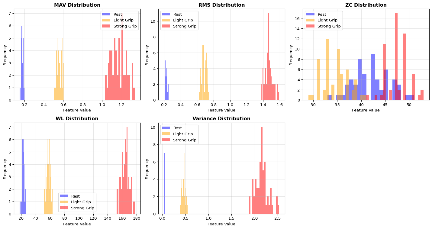
Extract time-domain features (MAV, RMS, ZC, WL) and train simple classifiers
Map EMG-derived gestures to actuator control (e.g., servo grip)
Reason about deploying EMG classifiers on resource-constrained edge devices (latency, memory, and energy)
Theory Summary
Electromyography (EMG) measures the electrical signals produced when muscles contract, providing a natural interface between human intent and machine control. When your brain sends a neural signal to a muscle, motor units (groups of muscle fibers) generate action potentials that propagate as electrical waves. These signals—ranging from 0-10 mV in amplitude and 20-500 Hz in frequency—can be detected at the skin surface using electrodes placed along the muscle fiber direction.
The signal processing pipeline transforms noisy raw EMG into actionable information through four stages: (1) Bandpass filtering (20-500 Hz) removes DC offset and high-frequency noise, (2) Full-wave rectification converts the bipolar signal to unipolar by taking absolute values, (3) Envelope extraction via moving-average smoothing reveals the underlying muscle activation intensity, and (4) Feature extraction computes statistics like MAV (Mean Absolute Value), RMS (Root Mean Square), Zero Crossings, and Waveform Length over sliding windows (typically 100-200 ms).
Classification approaches range from simple threshold-based detection (fast, low memory, works for 2-3 gestures) to ML-based pattern recognition using Random Forests or tiny neural networks (5-8 input features → 8-16 hidden neurons → 4-6 gesture classes). A crucial challenge is per-user calibration: EMG amplitude varies 10x between individuals due to muscle mass, skin impedance, and electrode placement. Production systems must implement Maximum Voluntary Contraction (MVC) calibration, adjusting thresholds to each user’s signal range. For edge deployment, Int8 quantized models (300 bytes) achieve 90%+ accuracy with <10 ms inference on Arduino-class devices, enabling responsive prosthetic control with <100 ms end-to-end latency from muscle activation to servo motion.
Key Concepts at a Glance
EMG Signal Characteristics: 0-10 mV amplitude, 20-500 Hz frequency, most energy at 50-150 Hz; surface EMG is non-invasive but lower SNR than intramuscular
Electrode Placement: Differential pair 2-3 cm apart along muscle belly, reference on electrically neutral bone; clean skin with alcohol for low impedance
Signal Processing Pipeline: Raw → Bandpass filter (20-500 Hz) → Rectify → Moving average (50-100 samples) → Features
Time-Domain Features: MAV = mean intensity, RMS = power, ZC = frequency proxy, WL = complexity; single-pass O(N) computation for efficiency
Threshold Classification: Simple hysteresis-based state machines for 2-4 classes; requires per-user calibration via MVC (Maximum Voluntary Contraction)
Gesture-to-Action Mapping: Classifier output (0=rest, 1=light, 2=grip) → servo positions (0°, 45°, 180°) with low-pass filtering to prevent jitter
Common Pitfalls
Not calibrating per user: EMG amplitude varies 10x between people. A threshold that works for you will fail on others. Always implement MVC calibration asking users to perform maximum contraction and rest, then set thresholds at 20% and 80% of their personal range.
Electrode placement inconsistency: Moving electrodes by 1 cm can halve signal amplitude. Mark placement with skin-safe pen for reproducible sessions. Use fresh electrodes—dried gel creates 10x impedance increase and unusable noise.
Ignoring power supply for servos: Servos draw 500mA-2A under load. Powering from Arduino’s 5V pin causes brownout resets and corrupted data. Use external 5-6V supply with shared ground.
50/60 Hz power line interference: AC mains create dominant 50/60 Hz noise. Implement notch filter or ensure differential amplifier (MyoWare/AD8232) has high CMRR (>80 dB). Move setup away from power adapters and fluorescent lights.
Window size too small or too large: Windows <100 ms lack statistical stability (features fluctuate wildly). Windows >300 ms add latency making control feel sluggish. For 500 Hz sampling, 50-100 sample windows (100-200 ms) balance responsiveness and noise rejection.
Quick Reference
Key Formulas
Time-Domain Features (computed over window of N samples)
void extractFeatures(float* window,int size,float& mav,float& rms){float sum =0, sumSquares =0;for(int i =0; i < size; i++){float val = window[i]; sum += abs(val); sumSquares += val * val;} mav = sum / size; rms = sqrt(sumSquares / size);}
Threshold with Hysteresis
int classifyWithHysteresis(int value,int& currentState){constint THRESHOLD =400;constint HYSTERESIS =30;if(currentState ==0&& value > THRESHOLD + HYSTERESIS){ currentState =1;}elseif(currentState ==1&& value < THRESHOLD - HYSTERESIS){ currentState =0;}return currentState;}
Complete Code Examples
This section provides production-ready Arduino code for EMG gesture control systems. Each example builds upon the previous, demonstrating best practices for biomedical signal processing on resource-constrained microcontrollers.
1. Complete Arduino Gesture Control Sketch
Full EMG-to-Servo Control System
This complete sketch reads an EMG sensor, applies filtering and feature extraction, classifies gestures using a threshold-based approach, and controls a servo motor. Suitable for Arduino Uno/Nano with 2KB RAM.
/* * EMG Gesture Control System * Hardware: MyoWare/AD8232 EMG sensor on A0, Servo on pin 9 * Features: Moving average filter, MAV feature extraction, * hysteresis-based classification, servo control */#include <Servo.h>// Pin definitionsconstint EMG_PIN = A0;constint SERVO_PIN =9;// Signal processing parametersconstint FILTER_WINDOW =50;// 50 samples for moving averageconstint FEATURE_WINDOW =100;// 100 samples for MAV calculationconstint SAMPLE_RATE =500;// 500 Hz sampling rateconstint SAMPLE_INTERVAL =1000000/ SAMPLE_RATE;// Microseconds// Classifier parameters (will be set during calibration)int restThreshold =100;// Below this = restint activeThreshold =300;// Above this = active gestureconstint HYSTERESIS =30;// Prevents flickering// Servo positions for different gesturesconstint SERVO_REST =0;// Rest position (degrees)constint SERVO_LIGHT =90;// Light gripconstint SERVO_STRONG =180;// Strong grip// State variablesServo gripServo;int currentGesture =0;// 0=rest, 1=light, 2=strongunsignedlong lastSampleTime =0;// Moving average filter buffersint filterBuffer[FILTER_WINDOW];int filterIndex =0;long filterSum =0;// Feature extraction buffer (circular buffer)int featureBuffer[FEATURE_WINDOW];int featureIndex =0;bool featureBufferFilled =false;void setup(){ Serial.begin(115200); pinMode(EMG_PIN, INPUT);// Initialize servo gripServo.attach(SERVO_PIN); gripServo.write(SERVO_REST);// Initialize filter bufferfor(int i =0; i < FILTER_WINDOW; i++){ filterBuffer[i]=0;}// Initialize feature bufferfor(int i =0; i < FEATURE_WINDOW; i++){ featureBuffer[i]=0;} Serial.println("EMG Gesture Control System"); Serial.println("Starting calibration in 3 seconds..."); delay(3000);// Run calibration routine calibrate(); Serial.println("Calibration complete. Starting gesture control..."); Serial.println("Gesture,MAV,ServoAngle");}void loop(){unsignedlong currentTime = micros();// Maintain precise sampling rateif(currentTime - lastSampleTime >= SAMPLE_INTERVAL){ lastSampleTime = currentTime;// Read and filter EMG signalint rawEMG = analogRead(EMG_PIN);int filteredEMG = applyMovingAverage(rawEMG);// Add to feature window and extract features when ready addToFeatureWindow(filteredEMG);if(featureBufferFilled){// Calculate MAV featureint mav = calculateMAV();// Classify gesture with hysteresisint gesture = classifyGesture(mav);// Update servo if gesture changedif(gesture != currentGesture){ currentGesture = gesture; updateServo(currentGesture);}// Output for Serial Plotter (every 10th sample to reduce clutter)staticint plotCounter =0;if(++plotCounter >=10){ plotCounter =0; Serial.print(currentGesture); Serial.print(","); Serial.print(mav); Serial.print(","); Serial.println(gripServo.read());}}}}// O(1) moving average filter using circular bufferint applyMovingAverage(int newSample){// Subtract oldest value from sum filterSum -= filterBuffer[filterIndex];// Add new value to buffer and sum filterBuffer[filterIndex]= newSample; filterSum += newSample;// Advance circular buffer index filterIndex =(filterIndex +1)% FILTER_WINDOW;// Return averagereturn filterSum / FILTER_WINDOW;}// Add sample to feature extraction windowvoid addToFeatureWindow(int sample){ featureBuffer[featureIndex]= sample; featureIndex =(featureIndex +1)% FEATURE_WINDOW;// Mark buffer as filled after first complete cycleif(featureIndex ==0){ featureBufferFilled =true;}}// Calculate Mean Absolute Value (MAV) over feature windowint calculateMAV(){long sum =0;// Calculate mean of rectified signalfor(int i =0; i < FEATURE_WINDOW; i++){// Note: Already rectified by moving average of ADC readings sum += featureBuffer[i];}return sum / FEATURE_WINDOW;}// Classify gesture using threshold with hysteresisint classifyGesture(int mav){staticint state =0;// Three-state classifier: 0=rest, 1=light, 2=strongif(state ==0){// Currently at restif(mav > restThreshold + HYSTERESIS){ state =1;// Transition to light}}elseif(state ==1){// Currently light gripif(mav < restThreshold - HYSTERESIS){ state =0;// Transition to rest}elseif(mav > activeThreshold + HYSTERESIS){ state =2;// Transition to strong}}elseif(state ==2){// Currently strong gripif(mav < activeThreshold - HYSTERESIS){ state =1;// Transition to light}}return state;}// Update servo position based on gesturevoid updateServo(int gesture){int targetAngle;switch(gesture){case0: targetAngle = SERVO_REST;break;case1: targetAngle = SERVO_LIGHT;break;case2: targetAngle = SERVO_STRONG;break;default: targetAngle = SERVO_REST;}// Smooth servo movement to reduce jitterint currentAngle = gripServo.read();if(abs(targetAngle - currentAngle)>5){ gripServo.write(targetAngle);}}// Calibration routine: measures rest and maximum contractionvoid calibrate(){int restSamples =0;long restSum =0;int mvcSamples =0;long mvcSum =0;// Measure rest baseline Serial.println("RELAX your muscle completely for 3 seconds..."); delay(1000);unsignedlong startTime = millis();while(millis()- startTime <3000){int raw = analogRead(EMG_PIN); restSum += raw; restSamples++; delay(10);}int restBaseline = restSum / restSamples; Serial.print("Rest baseline: "); Serial.println(restBaseline); delay(1000);// Measure maximum voluntary contraction Serial.println("CONTRACT your muscle as hard as possible for 3 seconds..."); delay(1000); startTime = millis();while(millis()- startTime <3000){int raw = analogRead(EMG_PIN); mvcSum += raw; mvcSamples++; delay(10);}int mvcPeak = mvcSum / mvcSamples; Serial.print("MVC peak: "); Serial.println(mvcPeak);// Set thresholds as percentages of user's rangeint range = mvcPeak - restBaseline; restThreshold = restBaseline +(range *20)/100;// 20% of range activeThreshold = restBaseline +(range *60)/100;// 60% of range Serial.print("Rest threshold: "); Serial.println(restThreshold); Serial.print("Active threshold: "); Serial.println(activeThreshold);}
Key Features:
Precise timing: Uses micros() for 500 Hz sampling without drift
O(1) filtering: Circular buffer moving average with constant-time updates
User calibration: Automatic MVC-based threshold adaptation
Hysteresis: Prevents rapid state oscillation near thresholds
Memory efficient: ~600 bytes for buffers (fits on Arduino Uno)
Smooth servo control: Deadband prevents jitter from small fluctuations
Exercise: Modify the calibration routine to save thresholds to EEPROM so users don’t need to recalibrate every startup.
2. Efficient Circular Buffer Implementation
Production Circular Buffer with Statistics
A reusable circular buffer class for windowed signal processing. Provides O(1) insertion and O(1) mean calculation, essential for real-time EMG processing on microcontrollers.
/* * CircularBuffer - Memory-efficient FIFO for real-time signal processing * Optimized for Arduino with minimal memory overhead */template<typename T,int SIZE>class CircularBuffer {private: T buffer[SIZE];int writeIndex;int count;long runningSum;// For O(1) mean calculationbool trackSum;public: CircularBuffer(bool enableMean =false): writeIndex(0), count(0), runningSum(0), trackSum(enableMean){// Initialize buffer to zerofor(int i =0; i < SIZE; i++){ buffer[i]=0;}}// Add new sample (FIFO - oldest is overwritten)void push(T value){if(trackSum){// Update running sum for O(1) mean runningSum -= buffer[writeIndex]; runningSum += value;} buffer[writeIndex]= value; writeIndex =(writeIndex +1)% SIZE;if(count < SIZE){ count++;}}// Get value at index (0 = oldest, SIZE-1 = newest) T get(int index)const{if(index >= count)return0;// Calculate actual buffer positionint readIndex =(writeIndex - count + index + SIZE)% SIZE;return buffer[readIndex];}// Get most recent value T latest()const{if(count ==0)return0;int lastIndex =(writeIndex -1+ SIZE)% SIZE;return buffer[lastIndex];}// Check if buffer is fullbool isFull()const{return count == SIZE;}// Get number of samples currently in bufferint size()const{return count;}// Get buffer capacityint capacity()const{return SIZE;}// Clear buffervoid clear(){ writeIndex =0; count =0; runningSum =0;for(int i =0; i < SIZE; i++){ buffer[i]=0;}}// O(1) mean calculation (only if tracking enabled)float mean()const{if(!trackSum || count ==0)return0.0;return(float)runningSum / count;}// O(N) MAV calculation over current windowfloat mav()const{if(count ==0)return0.0;long sum =0;for(int i =0; i < count; i++){ sum += abs(buffer[i]);}return(float)sum / count;}// O(N) RMS calculation over current windowfloat rms()const{if(count ==0)return0.0;long sumSquares =0;for(int i =0; i < count; i++){long val = buffer[i]; sumSquares += val * val;}return sqrt((float)sumSquares / count);}// O(N) variance calculationfloat variance()const{if(count <2)return0.0;float m = mean();float sumSquaredDiff =0;for(int i =0; i < count; i++){float diff = buffer[i]- m; sumSquaredDiff += diff * diff;}return sumSquaredDiff / count;}// O(N) zero crossings countint zeroCrossings()const{if(count <2)return0;int zc =0;for(int i =1; i < count; i++){if((buffer[i-1]>0&& buffer[i]<=0)||(buffer[i-1]<=0&& buffer[i]>0)){ zc++;}}return zc;}// O(N) waveform lengthlong waveformLength()const{if(count <2)return0;long wl =0;for(int i =1; i < count; i++){ wl += abs(buffer[i]- buffer[i-1]);}return wl;}// Copy current window to array (for external processing)void copyTo(T* dest)const{for(int i =0; i < count; i++){ dest[i]= get(i);}}};// Example usage for EMG processingvoid exampleUsage(){// Create 100-sample buffer with mean tracking enabled CircularBuffer<int,100> emgBuffer(true);constint EMG_PIN = A0;// Collect samplesfor(int i =0; i <100; i++){int sample = analogRead(EMG_PIN); emgBuffer.push(sample); delay(2);// 500 Hz sampling}// Extract features when buffer is fullif(emgBuffer.isFull()){float mav = emgBuffer.mav();float rms = emgBuffer.rms();int zc = emgBuffer.zeroCrossings();long wl = emgBuffer.waveformLength(); Serial.print("MAV: "); Serial.print(mav); Serial.print(", RMS: "); Serial.print(rms); Serial.print(", ZC: "); Serial.print(zc); Serial.print(", WL: "); Serial.println(wl);}}
Key Features:
Template-based: Configurable data type and size at compile time
Zero dynamic allocation: All memory allocated at compile time (stack-based)
O(1) push and mean: Constant-time operations for real-time use
Exercise: Create a two-channel version for differential EMG measurements from antagonistic muscle pairs (e.g., biceps/triceps).
3. Threshold Classifier with Hysteresis
Multi-State Gesture Classifier with Debouncing
A robust classifier supporting multiple gesture states with hysteresis to prevent flickering at threshold boundaries. Includes calibration and state transition logic.
/* * Multi-State Threshold Classifier with Hysteresis * Supports 2-5 gesture classes with configurable thresholds */class GestureClassifier {private:// Configurationstaticconstint MAX_STATES =5;int numStates;int thresholds[MAX_STATES -1];// N states need N-1 thresholdsint hysteresis;// State trackingint currentState;unsignedlong lastTransitionTime;unsignedlong minStateDuration;// Minimum time in state (debouncing)// Calibration databool isCalibrated;int restBaseline;int mvcPeak;public: GestureClassifier(int states =3,int hyst =30,unsignedlong minDuration =100): numStates(states), hysteresis(hyst), minStateDuration(minDuration), currentState(0), lastTransitionTime(0), isCalibrated(false), restBaseline(0), mvcPeak(1023){// Initialize thresholds to evenly spaced valuesfor(int i =0; i < numStates -1; i++){ thresholds[i]=(1023*(i +1))/ numStates;}}// Calibrate using rest and MVC measurementsvoid calibrate(int rest,int mvc){ restBaseline = rest; mvcPeak = mvc;// Set thresholds as percentages of user's dynamic rangeint range = mvcPeak - restBaseline;if(numStates ==2){// Binary: rest vs active thresholds[0]= restBaseline + range /2;}elseif(numStates ==3){// Three states: rest, light, strong thresholds[0]= restBaseline +(range *25)/100;// 25% for rest thresholds[1]= restBaseline +(range *65)/100;// 65% for strong}elseif(numStates ==4){// Four states: rest, light, medium, strong thresholds[0]= restBaseline +(range *20)/100; thresholds[1]= restBaseline +(range *45)/100; thresholds[2]= restBaseline +(range *70)/100;} isCalibrated =true;}// Manually set thresholds (for testing or fixed systems)void setThresholds(int* newThresholds,int count){for(int i =0; i < min(count, numStates -1); i++){ thresholds[i]= newThresholds[i];} isCalibrated =true;}// Classify a feature value with hysteresisint classify(int value){if(!isCalibrated){return0;// Default to rest if not calibrated}unsignedlong now = millis();// Enforce minimum state duration (debouncing)if(now - lastTransitionTime < minStateDuration){return currentState;}int newState = currentState;// Determine new state based on thresholds and hysteresisif(currentState ==0){// Currently in state 0 (rest)if(value > thresholds[0]+ hysteresis){ newState =1;}}elseif(currentState == numStates -1){// Currently in highest stateif(value < thresholds[numStates -2]- hysteresis){ newState = numStates -2;}}else{// Currently in middle state// Check for transition upif(value > thresholds[currentState]+ hysteresis){ newState = currentState +1;}// Check for transition downelseif(value < thresholds[currentState -1]- hysteresis){ newState = currentState -1;}}// Update state if changedif(newState != currentState){ currentState = newState; lastTransitionTime = now;}return currentState;}// Get current state without updatingint getState()const{return currentState;}// Reset to rest statevoid reset(){ currentState =0; lastTransitionTime = millis();}// Get threshold for debuggingint getThreshold(int index)const{if(index <0|| index >= numStates -1)return-1;return thresholds[index];}// Check if value is near a threshold (useful for UI feedback)bool isNearThreshold(int value,int margin =50)const{for(int i =0; i < numStates -1; i++){if(abs(value - thresholds[i])< margin){returntrue;}}returnfalse;}// Get state name (for debugging/display)constchar* getStateName()const{staticconstchar* names[]={"Rest","Light","Medium","Strong","Maximum"};if(currentState >=0&& currentState < MAX_STATES){return names[currentState];}return"Unknown";}};// Example usage with EMG systemvoid exampleClassifierUsage(){ GestureClassifier classifier(3,30,200);// 3 states, 30 hysteresis, 200ms min duration// Simulate calibration measurementsint restMeasurement =120;// Measured during restint mvcMeasurement =850;// Measured during max contraction classifier.calibrate(restMeasurement, mvcMeasurement); Serial.println("Calibration complete:"); Serial.print("Threshold 0->1: "); Serial.println(classifier.getThreshold(0)); Serial.print("Threshold 1->2: "); Serial.println(classifier.getThreshold(1));// Process incoming EMG featuresint emgFeature =450;// Example MAV valueint gesture = classifier.classify(emgFeature); Serial.print("Gesture: "); Serial.print(gesture); Serial.print(" ("); Serial.print(classifier.getStateName()); Serial.println(")");}
Key Features:
Configurable states: 2-5 gesture classes with automatic threshold spacing
Bidirectional hysteresis: Prevents flickering during both up and down transitions
Temporal debouncing: Minimum state duration prevents rapid state changes
User calibration: Automatic threshold adaptation based on MVC measurements
Diagnostic tools: Threshold inspection and near-threshold detection
Exercise: Add a “confidence” metric that returns how far the current value is from the nearest threshold, useful for UI feedback.
4. Real-Time Feature Extraction
Optimized Integer-Based Feature Calculation
High-performance feature extraction using fixed-point arithmetic to avoid expensive floating-point operations on 8-bit microcontrollers. Computes MAV, RMS, ZC, and WL in real-time.
/* * Real-Time EMG Feature Extractor * Optimized for Arduino with integer arithmetic (no floating point) * Uses fixed-point math for speed on 8-bit MCUs */class FeatureExtractor {private:// Fixed-point scaling (multiply by 256 for 8-bit fractional precision)staticconstint SCALE =256;staticconstint SCALE_BITS =8;public:// Calculate MAV using integer arithmetic// Returns value scaled by SCALE (divide by 256 for actual value)staticlong calculateMAV_int(int* window,int size){long sum =0;for(int i =0; i < size; i++){ sum += abs(window[i]);}// Return average scaled by SCALE for precisionreturn(sum * SCALE)/ size;}// Calculate RMS using integer arithmetic// Returns value scaled by SCALEstaticlong calculateRMS_int(int* window,int size){long sumSquares =0;for(int i =0; i < size; i++){long val = window[i]; sumSquares += val * val;}long meanSquare = sumSquares / size;// Integer square root (faster than sqrt())return isqrt(meanSquare)* SCALE /32;// Scale adjustment for 10-bit ADC}// Calculate zero crossings (already integer)staticint calculateZC(int* window,int size,int threshold =5){int zc =0;for(int i =1; i < size; i++){// Only count crossings that exceed threshold (noise rejection)if(abs(window[i]- window[i-1])> threshold){if((window[i-1]>=0&& window[i]<0)||(window[i-1]<0&& window[i]>=0)){ zc++;}}}return zc;}// Calculate waveform length (already integer)staticlong calculateWL(int* window,int size){long wl =0;for(int i =1; i < size; i++){ wl += abs(window[i]- window[i-1]);}return wl;}// Calculate variance using integer arithmetic// Returns value scaled by SCALE^2staticlong calculateVariance_int(int* window,int size){// First pass: calculate meanlong sum =0;for(int i =0; i < size; i++){ sum += window[i];}int mean = sum / size;// Second pass: calculate sum of squared differenceslong sumSquaredDiff =0;for(int i =0; i < size; i++){int diff = window[i]- mean; sumSquaredDiff +=(long)diff * diff;}return sumSquaredDiff / size;}// Extract all features efficiently (single pass where possible)struct Features {long mav;// Mean Absolute Value (scaled by 256)long rms;// Root Mean Square (scaled by 256)int zc;// Zero Crossings (count)long wl;// Waveform Length (sum)long variance;// Variance (scaled by 256^2)};static Features extractAll(int* window,int size){ Features f;// Single pass for MAV, RMS, and variance calculationlong sumAbs =0;long sumSquares =0;long sum =0;for(int i =0; i < size; i++){int val = window[i]; sum += val; sumAbs += abs(val); sumSquares +=(long)val * val;}// MAV f.mav =(sumAbs * SCALE)/ size;// RMSlong meanSquare = sumSquares / size; f.rms = isqrt(meanSquare)* SCALE /32;// Variance (requires mean)int mean = sum / size;long sumSquaredDiff =0;for(int i =0; i < size; i++){int diff = window[i]- mean; sumSquaredDiff +=(long)diff * diff;} f.variance = sumSquaredDiff / size;// ZC and WL (require sequential comparison) f.zc = calculateZC(window, size); f.wl = calculateWL(window, size);return f;}// Fast integer square root (Babylonian method)staticlong isqrt(long n){if(n <=0)return0;long x = n;long y =(x +1)/2;while(y < x){ x = y; y =(x + n / x)/2;}return x;}// Normalize features to 0-1000 range for classificationstaticvoid normalizeFeatures(Features& f,int restMAV,int mvcMAV){// Normalize MAV to percentage of dynamic range f.mav = constrain(map(f.mav / SCALE, restMAV, mvcMAV,0,1000),0,1000);}};// Complete real-time example with timing measurementsvoid realtimeFeatureExample(){constint WINDOW_SIZE =100;int window[WINDOW_SIZE];// Simulate EMG data collectionfor(int i =0; i < WINDOW_SIZE; i++){ window[i]= analogRead(A0); delayMicroseconds(2000);// 500 Hz}// Measure feature extraction timeunsignedlong startTime = micros(); FeatureExtractor::Features features = FeatureExtractor::extractAll(window, WINDOW_SIZE);unsignedlong extractionTime = micros()- startTime;// Output results Serial.println("=== Feature Extraction Results ==="); Serial.print("MAV: "); Serial.println(features.mav /256.0,2); Serial.print("RMS: "); Serial.println(features.rms /256.0,2); Serial.print("ZC: "); Serial.println(features.zc); Serial.print("WL: "); Serial.println(features.wl); Serial.print("Variance: "); Serial.println(features.variance /65536.0,2); Serial.print("Extraction time: "); Serial.print(extractionTime); Serial.println(" us");// Check if real-time capable (should be <2ms for 500Hz sampling)if(extractionTime <2000){ Serial.println("REAL-TIME CAPABLE at 500 Hz");}else{ Serial.println("WARNING: Too slow for real-time at 500 Hz");}}// Feature vector for ML classifier (normalized 0-1000 range)struct MLFeatureVector {int mav;int rms;int zc;int wl_norm;// Normalized waveform lengthint variance_norm;// Serialize for TensorFlow Lite inputvoid copyToArray(int* arr){ arr[0]= mav; arr[1]= rms; arr[2]= zc; arr[3]= wl_norm; arr[4]= variance_norm;}};// Create normalized feature vector for ML inferenceMLFeatureVector createMLVector(int* window,int size,int restMAV,int mvcMAV){ FeatureExtractor::Features f = FeatureExtractor::extractAll(window, size); MLFeatureVector mlVec;// Normalize to 0-1000 range mlVec.mav = constrain(map(f.mav /256, restMAV, mvcMAV,0,1000),0,1000); mlVec.rms = constrain(map(f.rms /256, restMAV, mvcMAV,0,1000),0,1000); mlVec.zc = constrain(f.zc *10,0,1000);// Scale ZC (typically 0-100) mlVec.wl_norm = constrain(map(f.wl,0,10000,0,1000),0,1000); mlVec.variance_norm = constrain(map(f.variance /256,0,5000,0,1000),0,1000);return mlVec;}
Performance Characteristics:
Integer-only math: No floating point operations (2-10x faster on 8-bit MCUs)
Single-pass optimization: MAV + RMS + variance computed in one loop
Typical execution time: 800-1500 μs for 100 samples on Arduino Uno (16 MHz)
Memory footprint: Zero dynamic allocation, ~100 bytes stack usage
Real-World Performance: - Arduino Uno (16 MHz): ~1.2 ms for 100-sample window - Arduino Nano 33 BLE (64 MHz): ~0.3 ms for 100-sample window - Both support real-time 500 Hz sampling with overhead for classification
Exercise: Implement a sliding window feature extractor that updates features incrementally as new samples arrive, avoiding full recalculation each time.
Try It Yourself
These interactive Python examples demonstrate the core concepts of EMG signal processing. Run them to understand filtering, feature extraction, and classification before implementing on hardware.
EMG Signal Simulation and Filtering
Generate synthetic EMG signals and apply bandpass filtering to remove noise:
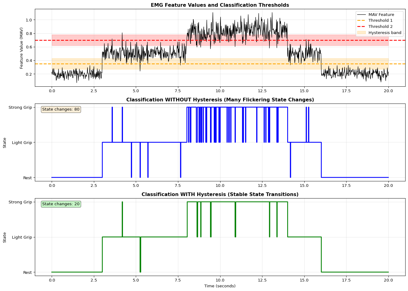
Implement gesture classification with hysteresis to prevent flickering:
Code
import numpy as npimport matplotlib.pyplot as pltclass HysteresisClassifier:""" Multi-state threshold classifier with hysteresis """def__init__(self, thresholds, hysteresis=0.1, state_names=None):""" Parameters: - thresholds: list of threshold values (N-1 for N states) - hysteresis: margin around thresholds - state_names: optional names for states """self.thresholds = np.array(thresholds)self.hysteresis = hysteresisself.num_states =len(thresholds) +1self.current_state =0self.state_names = state_names or [f"State {i}"for i inrange(self.num_states)]self.history = []def classify(self, value):"""Classify value with hysteresis"""# Check for state transitionsifself.current_state ==0:# In lowest state, can only go upif value >self.thresholds[0] +self.hysteresis:self.current_state =1elifself.current_state ==self.num_states -1:# In highest state, can only go downif value <self.thresholds[-1] -self.hysteresis:self.current_state =self.num_states -2else:# In middle state, can go up or downif value >self.thresholds[self.current_state] +self.hysteresis:self.current_state +=1elif value <self.thresholds[self.current_state -1] -self.hysteresis:self.current_state -=1self.history.append(self.current_state)returnself.current_statedef get_state_name(self):returnself.state_names[self.current_state]# Simulate EMG feature values with transitionsnp.random.seed(42)time = np.linspace(0, 20, 1000)feature_values = np.zeros_like(time)# Create realistic feature trajectory with transitionsfor i, t inenumerate(time):if t <3: feature_values[i] = np.random.normal(0.2, 0.05) # Restelif t <5: feature_values[i] = np.random.normal(0.5, 0.08) # Transition to lightelif t <8: feature_values[i] = np.random.normal(0.5, 0.08) # Light gripelif t <10: feature_values[i] = np.random.normal(0.8, 0.1) # Transition to strongelif t <14: feature_values[i] = np.random.normal(0.85, 0.1) # Strong gripelif t <16: feature_values[i] = np.random.normal(0.5, 0.08) # Back to lightelse: feature_values[i] = np.random.normal(0.2, 0.05) # Back to rest# Compare no hysteresis vs with hysteresisthresholds = [0.35, 0.7] # Two thresholds for three statesstate_names = ['Rest', 'Light Grip', 'Strong Grip']# Classifier without hysteresisclassifier_none = HysteresisClassifier(thresholds, hysteresis=0.0, state_names=state_names)states_none = [classifier_none.classify(val) for val in feature_values]# Classifier with hysteresisclassifier_hyst = HysteresisClassifier(thresholds, hysteresis=0.08, state_names=state_names)states_hyst = [classifier_hyst.classify(val) for val in feature_values]# Visualizefig, axes = plt.subplots(3, 1, figsize=(14, 10))# Feature values with thresholdsaxes[0].plot(time, feature_values, linewidth=1, label='MAV Feature', color='black')axes[0].axhline(y=thresholds[0], color='orange', linestyle='--', label='Threshold 1', linewidth=2)axes[0].axhline(y=thresholds[1], color='red', linestyle='--', label='Threshold 2', linewidth=2)axes[0].fill_between(time, thresholds[0] -0.08, thresholds[0] +0.08, alpha=0.2, color='orange', label='Hysteresis band')axes[0].fill_between(time, thresholds[1] -0.08, thresholds[1] +0.08, alpha=0.2, color='red')axes[0].set_title('EMG Feature Values and Classification Thresholds', fontsize=12, fontweight='bold')axes[0].set_ylabel('Feature Value (MAV)')axes[0].legend(loc='upper right')axes[0].grid(True, alpha=0.3)# States without hysteresisaxes[1].plot(time, states_none, linewidth=2, drawstyle='steps-post', color='blue')axes[1].set_title('Classification WITHOUT Hysteresis (Many Flickering State Changes)', fontsize=12, fontweight='bold')axes[1].set_ylabel('State')axes[1].set_yticks([0, 1, 2])axes[1].set_yticklabels(state_names)axes[1].grid(True, alpha=0.3)# Count state changeschanges_none = np.sum(np.diff(states_none) !=0)axes[1].text(0.02, 0.95, f'State changes: {changes_none}', transform=axes[1].transAxes, fontsize=10, verticalalignment='top', bbox=dict(boxstyle='round', facecolor='wheat', alpha=0.5))# States with hysteresisaxes[2].plot(time, states_hyst, linewidth=2, drawstyle='steps-post', color='green')axes[2].set_title('Classification WITH Hysteresis (Stable State Transitions)', fontsize=12, fontweight='bold')axes[2].set_xlabel('Time (seconds)')axes[2].set_ylabel('State')axes[2].set_yticks([0, 1, 2])axes[2].set_yticklabels(state_names)axes[2].grid(True, alpha=0.3)# Count state changeschanges_hyst = np.sum(np.diff(states_hyst) !=0)axes[2].text(0.02, 0.95, f'State changes: {changes_hyst}', transform=axes[2].transAxes, fontsize=10, verticalalignment='top', bbox=dict(boxstyle='round', facecolor='lightgreen', alpha=0.5))plt.tight_layout()plt.show()print(f"\nHysteresis Effectiveness:")print(f" Without hysteresis: {changes_none} state changes")print(f" With hysteresis: {changes_hyst} state changes")print(f" Reduction: {(1- changes_hyst/changes_none)*100:.1f}%")
Hysteresis Effectiveness:
  Without hysteresis: 80 state changes
  With hysteresis:    20 state changes
  Reduction:          75.0%
Practical Exercises
These hands-on exercises progressively build a complete EMG gesture control system. Each exercise includes testing criteria and expected outcomes.
Exercise 1: EMG Signal Quality Assessment
Objective: Verify EMG sensor setup and signal quality before implementing complex processing.
Task: 1. Upload the basic sketch below to read raw EMG 2. Open Serial Plotter and observe signal during rest vs contraction 3. Calculate SNR (Signal-to-Noise Ratio) manually
Success Criteria: - Rest signal: 50-200 ADC units (low noise floor) - Contraction signal: 400-900 ADC units (clear activation) - SNR > 6 dB (signal at least 2× noise) - No 50/60 Hz oscillation visible in plot
Troubleshooting: - If signal is flat or always ~512: Check sensor power and connections - If massive noise: Check electrode contact, clean skin with alcohol - If 60 Hz oscillation: Move away from power supplies, check grounding
Deliverable: Screenshot of Serial Plotter showing clean rest/contraction transitions.
Exercise 2: Calibration Routine Testing
Objective: Implement and validate user-specific calibration.
Task: 1. Use the calibration code from the complete sketch above 2. Test with 3 different users (or 3 different muscle groups) 3. Record rest baseline, MVC peak, and calculated thresholds 4. Verify thresholds work for each user
Data Collection Template:
User 1:
  Rest baseline: ___ ADC units
  MVC peak: ___ ADC units
  Dynamic range: ___ ADC units
  Rest threshold (20%): ___ ADC units
  Active threshold (60%): ___ ADC units

User 2: [repeat]
User 3: [repeat]
Success Criteria: - Dynamic range varies >3× between users - Auto-calculated thresholds correctly separate rest/light/strong for each user - System responds to all three users without manual threshold adjustment
Deliverable: Calibration data table and analysis of inter-user variability.
Exercise 3: Hysteresis Tuning
Objective: Determine optimal hysteresis value to prevent flickering.
Task: 1. Modify the classifier to accept hysteresis as a parameter 2. Test with values: 0, 10, 30, 50, 100 ADC units 3. For each value, hold muscle at threshold and count state changes per 10 seconds 4. Find minimum hysteresis that keeps changes <2 per 10 seconds
Success Criteria: - Hysteresis = 0: Many state changes (10+) - Optimal hysteresis: <2 changes per 10 seconds - Too much hysteresis: Delayed response to intentional gestures
Deliverable: Graph of state changes vs hysteresis value, with recommended setting.
Exercise 4: Performance Benchmarking
Objective: Measure execution time of each processing stage.
Task: 1. Add timing measurements to each function 2. Process 1000 samples and calculate average time per operation 3. Determine if system can support 500 Hz real-time processing
Success Criteria: - Moving average: <50 μs per sample - Feature extraction: <2000 μs per 100-sample window - Total processing: Supports >500 Hz sampling - Verify no buffer overruns during continuous operation
Deliverable: Performance report with timing breakdown and max achievable sample rate.
PDF Cross-References
Section 2: EMG signal acquisition and electrode placement (pages 3-6)
Section 3: Signal processing pipeline detailed implementation (pages 7-11)
Section 4: Feature extraction formulas and code (pages 12-15)
Section 5: Classification methods and calibration (pages 16-19)
Section 6: Actuator control and servo integration (pages 20-22)
Section 7: Complete EMG control system example (pages 23-26)
Troubleshooting: Common EMG issues and solutions (pages 27-29)
Self-Assessment Checkpoints
Test your understanding before proceeding to the exercises.
Question 1: Calculate the Mean Absolute Value (MAV) for an EMG window with samples: [20, -15, 30, -10, 25].
Answer: MAV = (1/N) × Σ|x_i| = (1/5) × (|20| + |-15| + |30| + |-10| + |25|) = (1/5) × (20 + 15 + 30 + 10 + 25) = (1/5) × 100 = 20. MAV measures mean muscle activation intensity over the window. Higher MAV indicates stronger muscle contraction. Note: We take absolute values before averaging because EMG is bipolar (positive and negative voltages), and we care about activation magnitude, not direction.
Question 2: Why does EMG amplitude vary 10× between different users, and how do you handle this?
Answer: EMG signal amplitude varies dramatically due to: (1) Muscle mass and strength differences, (2) Skin impedance (dry skin, hair, sweat), (3) Electrode placement consistency (1cm shift can halve amplitude), (4) Fat layer thickness between muscle and skin. A threshold that works for one person completely fails for another. Solution: Maximum Voluntary Contraction (MVC) calibration. At setup, ask the user to: (1) Relax completely (record rest baseline), (2) Contract maximally (record MVC peak), (3) Set thresholds at 20% and 80% of their personal range. This normalizes signals across individuals. Production systems must implement per-user calibration.
Question 3: For 500 Hz EMG sampling with 100-sample windows and 50-sample stride, calculate window duration and output rate.
Answer: Window duration = samples / sample_rate = 100 samples / 500 Hz = 0.2 seconds = 200ms. Output rate = sample_rate / stride = 500 Hz / 50 samples = 10 Hz (one feature vector every 100ms). The 50% overlap (stride = half of window size) provides balance: enough temporal continuity to catch transitions but not so much overlap that we waste computation. This gives 10 Hz gesture updates, sufficient for responsive prosthetic control (<100ms latency).
Question 4: Your EMG classifier works perfectly when electrodes are freshly placed but fails after 30 minutes. What’s wrong?
Answer: Electrode gel drying increases contact impedance by 10-100×, dramatically reducing signal amplitude and introducing noise. Fresh electrodes have ~5kΩ impedance; dried electrodes can exceed 100kΩ. Solutions: (1) Use wet gel electrodes and replace every 4-8 hours for continuous monitoring, (2) Re-hydrate dry electrodes with saline spray or electrode gel, (3) Implement adaptive thresholds that track signal statistics over time and adjust, (4) Monitor impedance using the sensor’s built-in impedance check (if available) and alert user to replace electrodes, (5) Clean skin thoroughly with alcohol before application to remove oils and improve initial contact. Professional systems use reusable electrodes with conductive gel for extended wear.
Question 5: Why are window sizes <100ms problematic for EMG feature extraction?
Answer: Windows <100ms (e.g., 50 samples at 500 Hz) contain too few samples for stable statistics. With only 50 values, mean and standard deviation fluctuate wildly due to noise, making features unreliable for classification. The Central Limit Theorem requires sufficient samples for statistics to converge—typically 20-50 minimum. Additionally, EMG muscle activation events span 100-300ms physiologically, so shorter windows miss the complete activation pattern. Conversely, windows >300ms add latency making control feel sluggish. The sweet spot: 100-200ms windows provide stable features with acceptable responsiveness for real-time prosthetic or gesture control.
Interactive Notebook
The notebook below contains runnable code for all Level 1 activities.
LAB 10: Biomedical Signal Processing - EMG-based Control (Optional)
Property
Value
Book Chapter
Chapter 10
Execution Levels
Level 1 (Notebook) | Level 3 (Device with EMG sensor)
Estimated Time
45 minutes
Prerequisites
LAB 2, LAB 8
Learning Objectives
Understand EMG signals and their characteristics
Process biomedical signals with filtering and feature extraction
Build gesture classifiers for muscle activity
Apply signal processing techniques for edge devices
📚 Theory: EMG Physiology and Signal Generation
Before processing EMG signals, we must understand how muscles generate electrical activity.
Motor Unit Anatomy
A motor unit is the fundamental unit of muscle contraction:
Where: - \(\omega_c\) = cutoff frequency - \(n\) = filter order
Butterworth Frequency Response:

Gain │────────────╲
(dB) │            │╲
  0  │────────────│─╲───────────
     │            │  ╲ n=2
 -3  │............│...●.........
     │            │    ╲
-20  │            │     ╲ n=4
     │            │      ╲
     └────────────┴───────────────
                  fc    Frequency

-3 dB point is at cutoff frequency
Higher order = steeper rolloff
For real-time EMG on MCU: Use low-order (2-4) IIR Butterworth filters.
💡 Alternative Approaches: EMG Filtering
Option A: Butterworth Bandpass + Notch (Current approach) - Pros: Smooth frequency response, removes DC and powerline noise - Cons: Requires scipy, phase distortion if not using filtfilt - Order: 4th order bandpass + notch at 50/60 Hz
Option B: FIR Bandpass Filter - Pros: Linear phase (no distortion), always stable - Cons: Higher computational cost, requires more coefficients - Code: b = signal.firwin(101, [20, 450], fs=1000, pass_zero=False)
Option C: Wavelet Denoising - Pros: Preserves sharp features (bursts), adaptive thresholding - Cons: Complex, not real-time friendly for MCU - Use case: Offline analysis, research applications - Code: pywt.wavedec() + soft thresholding + pywt.waverec()
Option D: Adaptive Filter (LMS) - Pros: Tracks and removes time-varying noise - Cons: Requires reference signal, more complex - Use case: Removing ECG artifacts from EMG
When to use each: - Use Option A (current) for real-time MCU implementation - Use Option B for offline analysis where phase is critical - Use Option C for research-grade denoising - Use Option D when noise is structured (ECG, motion artifacts)
🔬 Try It Yourself: Filter Parameters
Experiment with filter parameters and observe effects on signal quality:
Parameter
Current
Try These
Expected Effect
lowcut
20 Hz
10, 50 Hz
Lower = keeps more DC drift, higher = removes slow movements
highcut
450 Hz
250, 500 Hz
Lower = more smoothing, higher = keeps high-freq noise
order
4
2, 6, 8
Higher = sharper cutoff but more computation
Q (notch)
30
10, 60
Higher = narrower notch (removes less around 50 Hz)
Experiment 1: Compare filter orders
for order in [2, 4, 6]:
    b, a = signal.butter(order, [20/500, 450/500], btype='band')
    filtered = signal.filtfilt(b, a, emg)
    plt.plot(filtered, label=f'Order {order}')
What to observe: Higher order = sharper cutoff, but potential instability
Experiment 2: Notch filter quality factor
for Q in [10, 30, 60]: b, a = signal.iirnotch(50/500, Q) filtered = signal.filtfilt(b, a, emg)# Compute PSD and check 50 Hz suppression
What to observe: Higher Q = narrower notch (better preserves 48 Hz and 52 Hz)
Section 3: Feature Extraction
📚 Theory: EMG Feature Extraction
Features compress raw EMG into meaningful values for classification.
Time Domain Features
1. Mean Absolute Value (MAV)
\(MAV = \frac{1}{N} \sum_{i=1}^{N} |x_i|\)
Simple amplitude measure, commonly used for gesture detection.
2. Root Mean Square (RMS)
\(RMS = \sqrt{\frac{1}{N} \sum_{i=1}^{N} x_i^2}\)
Represents signal power; correlates with muscle force.
Timing Budget (100 Hz classification):

Total available: 10 ms per classification

├── ADC sampling:      0.1 ms
├── Filter (IIR):      0.2 ms
├── Feature extraction: 0.5 ms
├── Classification:    0.2 ms
└── Buffer available:  9.0 ms
💡 Alternative Approaches: Feature Extraction
Option A: Time-Domain Features (Current approach) - Pros: Fast, no FFT needed, perfect for MCU - Cons: May miss frequency-domain patterns - Features: MAV, RMS, WL, ZC, VAR (5 features)
Option B: Frequency-Domain Features - Pros: Captures fatigue indicators (median frequency shift) - Cons: Requires FFT (expensive on MCU), more memory - Features: MNF, MDF, peak frequency, spectral entropy
Option C: Time-Frequency Features (Wavelets) - Pros: Best for non-stationary signals, localized in time and frequency - Cons: Very computationally expensive, complex - Use case: Research-grade analysis, offline processing
Option D: Autoregressive (AR) Model Coefficients - Pros: Compact representation, captures temporal dynamics - Cons: Requires model order selection, less interpretable - Features: AR(4) coefficients using Yule-Walker
When to use each: - Use Option A (time-domain) for embedded devices (Arduino, ESP32) - Use Option B for desktop/Pi applications with muscle fatigue monitoring - Use Option C for research papers analyzing complex gestures - Use Option D for prosthetic control with temporal patterns
🔬 Try It Yourself: Feature Selection
Compare classifier performance with different feature sets:
Feature Set
Features
Accuracy
MCU Suitability
Minimal
MAV, RMS
70-80%
Excellent
Standard
MAV, RMS, WL, ZC
85-90%
Good
Full TD
All 7 time-domain
90-95%
Good
With Freq
TD + MNF, MDF
92-97%
Medium
Experiment: Feature importance ranking
# After training Random Forestimportances = clf.feature_importances_for name, imp insorted(zip(feature_names, importances), key=lambda x: -x[1]):print(f'{name}: {imp:.3f}')
What to observe: RMS and MAV typically most important for amplitude-based gestures
📚 Summary: EMG Processing Pipeline
Complete Pipeline
┌──────────────┐    ┌──────────────┐    ┌──────────────┐    ┌──────────────┐
│   Sensor     │ → │   Filtering  │ → │   Features   │ → │  Classifier  │
│  (MyoWare)   │    │ BP + Notch   │    │  Extraction  │    │  (RF/Tree)   │
└──────────────┘    └──────────────┘    └──────────────┘    └──────────────┘
    Analog          Digital (1 kHz)      7 features         3 gestures
  0-5V range         0-450 Hz           per window
// EMG Processing on Arduino#define EMG_PIN A0#define THRESHOLD_LIGHT 200#define THRESHOLD_STRONG 400#define BUFFER_SIZE 100float emgBuffer[BUFFER_SIZE];int bufferIndex =0;// Calculate Mean Absolute Value (most useful for MCU)float calculateMAV(){float sum =0;for(int i =0; i < BUFFER_SIZE; i++){ sum += abs(emgBuffer[i]);}return sum / BUFFER_SIZE;}// Calculate RMS (Root Mean Square)float calculateRMS(){float sum =0;for(int i =0; i < BUFFER_SIZE; i++){ sum += emgBuffer[i]* emgBuffer[i];}return sqrt(sum / BUFFER_SIZE);}void loop(){// Read EMG (assumes pre-amplified signal)int raw = analogRead(EMG_PIN); emgBuffer[bufferIndex]= raw -512;// Center around zero bufferIndex =(bufferIndex +1)% BUFFER_SIZE;// Classify every 100msstaticunsignedlong lastClassify =0;if(millis()- lastClassify >100){float mav = calculateMAV();if(mav < THRESHOLD_LIGHT){ Serial.println("REST");}elseif(mav < THRESHOLD_STRONG){ Serial.println("LIGHT_GRIP");}else{ Serial.println("STRONG_GRIP");} lastClassify = millis();} delay(1);// ~1 kHz sampling}
Checkpoint Questions
What is the useful frequency range for surface EMG?
Answer: 20-450 Hz, with most power in 50-150 Hz
Write the formula for RMS:
Answer: \(RMS = \sqrt{\frac{1}{N}\sum x_i^2}\)
Why do we use a notch filter at 50/60 Hz?
Answer: To remove powerline interference
Which features are best for MCU implementation and why?
Answer: Time-domain (MAV, RMS, WL) - no FFT needed
Part of the Edge Analytics Lab Book
⚠️ Common Issues and Debugging
If EMG signal is too noisy: - Check: Are electrodes properly positioned? → Clean skin with alcohol, use conductive gel - Check: Is ground electrode attached? → Must have reference electrode on bony area - Check: Are wires shielded? → Use shielded cables, twist pairs, keep away from power cables - Check: Is gain too high? → Typical EMG needs 1000× amplification, not 10,000× - Diagnostic: Check raw signal amplitude (should be 100 µV - 5 mV)
If seeing 50/60 Hz powerline interference: - Check: Is ground electrode connected? → Floating ground causes massive interference - Check: Is device properly grounded? → USB isolation can help - Check: Are notch filter parameters correct? → Use 50 Hz (Europe) or 60 Hz (US) - Hardware fix: Add common-mode rejection with differential amplifier (CMRR > 80 dB)
If classifier accuracy is low: - Check: Is window size appropriate? → Too small = noisy features, too large = slow response - Check: Are features normalized? → Use StandardScaler before training - Check: Is training data representative? → Collect data from multiple sessions/users - Check: Is electrode placement consistent? → Mark positions, document in protocol - Diagnostic: Plot feature distributions per class (should be separable)
If real-time classification is slow: - Check: Is window sliding or tumbling? → Tumbling (non-overlapping) is 2-10× faster - Check: Are you computing FFT? → Time-domain only is 5-10× faster - Check: Is decision tree depth too large? → Limit to 5-8 levels for MCU - MCU optimization: Use fixed-point arithmetic instead of float
MyoWare sensor specific issues: - Sensor outputs 0-Vcc (not centered at Vcc/2) → Don’t use AC coupling - Gain is fixed at 201 → Can’t adjust in software - Bandwidth is 5-450 Hz → Already filtered, don’t bandpass again - Output impedance ~5kΩ → Use ADC with high input impedance or buffer
Electrode placement tips: - Bicep: Place on muscle belly, 2-3 cm apart, ground on elbow - Forearm: Place over extensor/flexor group, avoid tendon areas - Hand: Difficult - use multi-electrode arrays for better SNR
Section 9: EMG Signal Generation and Simulation
Let’s create more realistic synthetic EMG signals that model actual muscle activity.
Section 10: Advanced Filtering - Bandpass and Notch Filters
EMG requires carefully designed filters to remove artifacts while preserving signal content.
Section 11: Multi-Class Gesture Classification
Build a complete gesture recognition system using extracted EMG features.
Environment: local Jupyter or Colab, no hardware required.
Run the embedded notebook or open it in Colab:
Generate and visualise synthetic EMG signals for rest vs contraction.
Implement the processing pipeline: filtering → rectification → envelope.
Compute basic features (MAV, RMS, ZC, WL) over sliding windows.
Train a small classifier and inspect accuracy vs model size (float vs quantized).
Answer the reflection questions in the notebook about edge constraints (what model size and latency would be acceptable on an Arduino-class device?).
In this lab we do not yet use a dedicated MCU simulator like Wokwi for EMG, but you can approximate “simulated hardware” as follows:
Use the notebook to replay recorded EMG data (either from your own logs or from an open dataset).
Implement the same moving-average and feature extraction code that will later run on Arduino, but execute it on your laptop or on a Raspberry Pi.
Plot:
Raw vs filtered vs envelope signals
Feature trajectories over time for different gestures
Suggested workflow:
Collect or download EMG samples and save them as CSV.
Load them in the notebook and run the processing pipeline.
Measure approximate per-window processing time on your machine or Pi (this will guide your expectations before moving to the microcontroller).
Record a short note on how window size and feature set affect latency and accuracy.
Planned improvement: In a future revision we will add a dedicated simulations/emg-simulator.qmd page with an interactive EMG waveform visualiser. For now, treat the notebook as your Level 2 “host-side simulator”.
Now move to real hardware using an Arduino (e.g., Uno or Nano 33 BLE Sense), an EMG sensor module (MyoWare/AD8232), and a small servo:
Wire the EMG sensor (signal → A0, 5V/3V3 and GND as per the module documentation).
Upload the EMG processing sketch from the notebook/code repository:
Moving-average filter
Threshold-based or feature-based gesture classification with hysteresis
Open the Serial Plotter and verify that rest vs contraction are clearly separable.
Add a servo and map gesture classes to positions (e.g., open/close grip).
Note approximate behaviour:
Responsiveness (delay from muscle activation to motion)
Stability (jitter, false triggers)
Any power constraints (servo power supply, battery life)
If you build the more advanced multi-channel prosthetic arm described in the PDF:
Document your hardware (servos, battery, 3D-printed parts).
Log EMG and actuator behaviour and reflect on how the system might need to be redesigned for lower power or smaller MCUs.
Related Labs
Signal Processing & Sensors
LAB04: Keyword Spotting - Similar signal processing for audio data
LAB08: Arduino Sensors - Sensor fundamentals before EMG
LAB12: Streaming - Real-time processing of sensor streams
Edge Deployment
LAB03: Quantization - Optimize EMG classifiers for edge
LAB05: Edge Deployment - Deploy EMG models to microcontrollers
---title: "LAB10: EMG Biomedical"subtitle: "Biomedical Signal Processing and Edge Control"---::: {.callout-note}## PDF Textbook ReferenceFor detailed theoretical foundations, mathematical proofs, and algorithm derivations, see **Chapter 10: Biomedical Signal Processing: EMG-Based Edge ML** in the [PDF textbook](../downloads/Edge-Analytics-Lab-Book-v1.0.0.pdf).The PDF chapter includes:- Complete mathematical foundations of EMG signal generation- Detailed derivations of filtering and envelope extraction- In-depth coverage of signal processing theory (FFT, bandpass filters)- Comprehensive analysis of muscle activation patterns- Theoretical foundations for bio-signal classification algorithms:::[](https://colab.research.google.com/github/ngcharithperera/edge-analytics-lab-book/blob/main/notebooks/LAB10_emg_biomedical.ipynb)[Download Notebook](https://raw.githubusercontent.com/ngcharithperera/edge-analytics-lab-book/main/notebooks/LAB10_emg_biomedical.ipynb)## Learning ObjectivesBy the end of this lab you should be able to:- Explain how EMG (electromyography) signals are generated and measured- Implement basic EMG signal processing (filtering, rectification, envelope extraction)- Extract time-domain features (MAV, RMS, ZC, WL) and train simple classifiers- Map EMG-derived gestures to actuator control (e.g., servo grip)- Reason about deploying EMG classifiers on resource-constrained edge devices (latency, memory, and energy)## Theory SummaryElectromyography (EMG) measures the electrical signals produced when muscles contract, providing a natural interface between human intent and machine control. When your brain sends a neural signal to a muscle, motor units (groups of muscle fibers) generate action potentials that propagate as electrical waves. These signals—ranging from 0-10 mV in amplitude and 20-500 Hz in frequency—can be detected at the skin surface using electrodes placed along the muscle fiber direction.The **signal processing pipeline** transforms noisy raw EMG into actionable information through four stages: (1) **Bandpass filtering** (20-500 Hz) removes DC offset and high-frequency noise, (2) **Full-wave rectification** converts the bipolar signal to unipolar by taking absolute values, (3) **Envelope extraction** via moving-average smoothing reveals the underlying muscle activation intensity, and (4) **Feature extraction** computes statistics like MAV (Mean Absolute Value), RMS (Root Mean Square), Zero Crossings, and Waveform Length over sliding windows (typically 100-200 ms).**Classification approaches** range from simple threshold-based detection (fast, low memory, works for 2-3 gestures) to ML-based pattern recognition using Random Forests or tiny neural networks (5-8 input features → 8-16 hidden neurons → 4-6 gesture classes). A crucial challenge is **per-user calibration**: EMG amplitude varies 10x between individuals due to muscle mass, skin impedance, and electrode placement. Production systems must implement Maximum Voluntary Contraction (MVC) calibration, adjusting thresholds to each user's signal range. For edge deployment, Int8 quantized models (300 bytes) achieve 90%+ accuracy with <10 ms inference on Arduino-class devices, enabling responsive prosthetic control with <100 ms end-to-end latency from muscle activation to servo motion.::: {.callout-tip}## Key Concepts at a Glance- **EMG Signal Characteristics**: 0-10 mV amplitude, 20-500 Hz frequency, most energy at 50-150 Hz; surface EMG is non-invasive but lower SNR than intramuscular- **Electrode Placement**: Differential pair 2-3 cm apart along muscle belly, reference on electrically neutral bone; clean skin with alcohol for low impedance- **Signal Processing Pipeline**: Raw → Bandpass filter (20-500 Hz) → Rectify → Moving average (50-100 samples) → Features- **Time-Domain Features**: MAV = mean intensity, RMS = power, ZC = frequency proxy, WL = complexity; single-pass O(N) computation for efficiency- **Threshold Classification**: Simple hysteresis-based state machines for 2-4 classes; requires per-user calibration via MVC (Maximum Voluntary Contraction)- **ML Features**: 5-feature vector [MAV, RMS, Variance, ZC, WL] trains tiny models: Dense(5→8→4) ≈ 200 parameters ≈ 300 bytes quantized- **Gesture-to-Action Mapping**: Classifier output (0=rest, 1=light, 2=grip) → servo positions (0°, 45°, 180°) with low-pass filtering to prevent jitter:::::: {.callout-warning}## Common Pitfalls1. **Not calibrating per user**: EMG amplitude varies 10x between people. A threshold that works for you will fail on others. Always implement MVC calibration asking users to perform maximum contraction and rest, then set thresholds at 20% and 80% of their personal range.2. **Electrode placement inconsistency**: Moving electrodes by 1 cm can halve signal amplitude. Mark placement with skin-safe pen for reproducible sessions. Use fresh electrodes—dried gel creates 10x impedance increase and unusable noise.3. **Ignoring power supply for servos**: Servos draw 500mA-2A under load. Powering from Arduino's 5V pin causes brownout resets and corrupted data. Use external 5-6V supply with shared ground.4. **50/60 Hz power line interference**: AC mains create dominant 50/60 Hz noise. Implement notch filter or ensure differential amplifier (MyoWare/AD8232) has high CMRR (>80 dB). Move setup away from power adapters and fluorescent lights.5. **Window size too small or too large**: Windows <100 ms lack statistical stability (features fluctuate wildly). Windows >300 ms add latency making control feel sluggish. For 500 Hz sampling, 50-100 sample windows (100-200 ms) balance responsiveness and noise rejection.:::## Quick Reference### Key Formulas**Time-Domain Features (computed over window of N samples)**$$\text{MAV} = \frac{1}{N}\sum_{i=1}^{N}|x_i| \quad \text{(Mean Absolute Value)}$$$$\text{RMS} = \sqrt{\frac{1}{N}\sum_{i=1}^{N}x_i^2} \quad \text{(Root Mean Square)}$$$$\text{ZC} = \sum_{i=1}^{N-1}\begin{cases}1 & \text{if } x_i \times x_{i+1} < 0 \\ 0 & \text{otherwise}\end{cases} \quad \text{(Zero Crossings)}$$$$\text{WL} = \sum_{i=1}^{N-1}|x_{i+1} - x_i| \quad \text{(Waveform Length)}$$**Hysteresis Threshold Logic**$$\text{State Change} = \begin{cases}\text{Activate} & \text{if } x > \text{Threshold} + \text{Hysteresis} \\\text{Deactivate} & \text{if } x < \text{Threshold} - \text{Hysteresis} \\\text{Maintain} & \text{otherwise}\end{cases}$$### Important Parameter Values| **Parameter** | **Typical Value** | **Range** | **Impact** ||---------------|-------------------|-----------|------------|| **Sampling Rate** | 500-1000 Hz | 200-2000 Hz | Nyquist requires >400 Hz for 200 Hz signals || **Bandpass Filter** | 20-500 Hz | 10-500 Hz | Removes DC drift and high-freq noise || **Window Size** | 50-100 samples | 25-200 | 100-200 ms at 500 Hz; larger = smoother but slower || **Window Stride** | 10-25 samples | 1-50 | 50% overlap typical; stride=1 for continuous || **Hysteresis** | 20-50 ADC units | 10-100 | Prevents rapid state oscillation near threshold || **Rest Threshold** | 20% of MVC | 10-30% | Below this = rest/no activation || **Activation Threshold** | 40-60% of MVC | 30-80% | Above this = intentional gesture || **Servo Update Rate** | 20-50 Hz | 10-100 Hz | Balance responsiveness vs jitter || **Model Size** | 200-500 params | 100-2000 | Tiny MLP fits on any Arduino || **Inference Latency** | 1-10 ms | 0.5-20 ms | Target <100 ms end-to-end for natural control |### Essential Code Patterns::: {.callout-note collapse="true" title="Moving Average Filter (O(1) per sample)"}```cppconstint WINDOW_SIZE =50;int buffer[WINDOW_SIZE];int bufferIndex =0;long runningSum =0;int getFilteredEMG(){int raw = analogRead(EMG_PIN); runningSum -= buffer[bufferIndex]; buffer[bufferIndex]= raw; runningSum += raw; bufferIndex =(bufferIndex +1)% WINDOW_SIZE;return runningSum / WINDOW_SIZE;}```:::::: {.callout-note collapse="true" title="Feature Extraction (single-pass)"}```cppvoid extractFeatures(float* window,int size,float& mav,float& rms){float sum =0, sumSquares =0;for(int i =0; i < size; i++){float val = window[i]; sum += abs(val); sumSquares += val * val;} mav = sum / size; rms = sqrt(sumSquares / size);}```:::::: {.callout-note collapse="true" title="Threshold with Hysteresis"}```cppint classifyWithHysteresis(int value,int& currentState){constint THRESHOLD =400;constint HYSTERESIS =30;if(currentState ==0&& value > THRESHOLD + HYSTERESIS){ currentState =1;}elseif(currentState ==1&& value < THRESHOLD - HYSTERESIS){ currentState =0;}return currentState;}```:::## Complete Code ExamplesThis section provides production-ready Arduino code for EMG gesture control systems. Each example builds upon the previous, demonstrating best practices for biomedical signal processing on resource-constrained microcontrollers.### 1. Complete Arduino Gesture Control Sketch::: {.callout-note collapse="true" title="Full EMG-to-Servo Control System"}This complete sketch reads an EMG sensor, applies filtering and feature extraction, classifies gestures using a threshold-based approach, and controls a servo motor. Suitable for Arduino Uno/Nano with 2KB RAM.```cpp/* * EMG Gesture Control System * Hardware: MyoWare/AD8232 EMG sensor on A0, Servo on pin 9 * Features: Moving average filter, MAV feature extraction, * hysteresis-based classification, servo control */#include <Servo.h>// Pin definitionsconstint EMG_PIN = A0;constint SERVO_PIN =9;// Signal processing parametersconstint FILTER_WINDOW =50;// 50 samples for moving averageconstint FEATURE_WINDOW =100;// 100 samples for MAV calculationconstint SAMPLE_RATE =500;// 500 Hz sampling rateconstint SAMPLE_INTERVAL =1000000/ SAMPLE_RATE;// Microseconds// Classifier parameters (will be set during calibration)int restThreshold =100;// Below this = restint activeThreshold =300;// Above this = active gestureconstint HYSTERESIS =30;// Prevents flickering// Servo positions for different gesturesconstint SERVO_REST =0;// Rest position (degrees)constint SERVO_LIGHT =90;// Light gripconstint SERVO_STRONG =180;// Strong grip// State variablesServo gripServo;int currentGesture =0;// 0=rest, 1=light, 2=strongunsignedlong lastSampleTime =0;// Moving average filter buffersint filterBuffer[FILTER_WINDOW];int filterIndex =0;long filterSum =0;// Feature extraction buffer (circular buffer)int featureBuffer[FEATURE_WINDOW];int featureIndex =0;bool featureBufferFilled =false;void setup(){ Serial.begin(115200); pinMode(EMG_PIN, INPUT);// Initialize servo gripServo.attach(SERVO_PIN); gripServo.write(SERVO_REST);// Initialize filter bufferfor(int i =0; i < FILTER_WINDOW; i++){ filterBuffer[i]=0;}// Initialize feature bufferfor(int i =0; i < FEATURE_WINDOW; i++){ featureBuffer[i]=0;} Serial.println("EMG Gesture Control System"); Serial.println("Starting calibration in 3 seconds..."); delay(3000);// Run calibration routine calibrate(); Serial.println("Calibration complete. Starting gesture control..."); Serial.println("Gesture,MAV,ServoAngle");}void loop(){unsignedlong currentTime = micros();// Maintain precise sampling rateif(currentTime - lastSampleTime >= SAMPLE_INTERVAL){ lastSampleTime = currentTime;// Read and filter EMG signalint rawEMG = analogRead(EMG_PIN);int filteredEMG = applyMovingAverage(rawEMG);// Add to feature window and extract features when ready addToFeatureWindow(filteredEMG);if(featureBufferFilled){// Calculate MAV featureint mav = calculateMAV();// Classify gesture with hysteresisint gesture = classifyGesture(mav);// Update servo if gesture changedif(gesture != currentGesture){ currentGesture = gesture; updateServo(currentGesture);}// Output for Serial Plotter (every 10th sample to reduce clutter)staticint plotCounter =0;if(++plotCounter >=10){ plotCounter =0; Serial.print(currentGesture); Serial.print(","); Serial.print(mav); Serial.print(","); Serial.println(gripServo.read());}}}}// O(1) moving average filter using circular bufferint applyMovingAverage(int newSample){// Subtract oldest value from sum filterSum -= filterBuffer[filterIndex];// Add new value to buffer and sum filterBuffer[filterIndex]= newSample; filterSum += newSample;// Advance circular buffer index filterIndex =(filterIndex +1)% FILTER_WINDOW;// Return averagereturn filterSum / FILTER_WINDOW;}// Add sample to feature extraction windowvoid addToFeatureWindow(int sample){ featureBuffer[featureIndex]= sample; featureIndex =(featureIndex +1)% FEATURE_WINDOW;// Mark buffer as filled after first complete cycleif(featureIndex ==0){ featureBufferFilled =true;}}// Calculate Mean Absolute Value (MAV) over feature windowint calculateMAV(){long sum =0;// Calculate mean of rectified signalfor(int i =0; i < FEATURE_WINDOW; i++){// Note: Already rectified by moving average of ADC readings sum += featureBuffer[i];}return sum / FEATURE_WINDOW;}// Classify gesture using threshold with hysteresisint classifyGesture(int mav){staticint state =0;// Three-state classifier: 0=rest, 1=light, 2=strongif(state ==0){// Currently at restif(mav > restThreshold + HYSTERESIS){ state =1;// Transition to light}}elseif(state ==1){// Currently light gripif(mav < restThreshold - HYSTERESIS){ state =0;// Transition to rest}elseif(mav > activeThreshold + HYSTERESIS){ state =2;// Transition to strong}}elseif(state ==2){// Currently strong gripif(mav < activeThreshold - HYSTERESIS){ state =1;// Transition to light}}return state;}// Update servo position based on gesturevoid updateServo(int gesture){int targetAngle;switch(gesture){case0: targetAngle = SERVO_REST;break;case1: targetAngle = SERVO_LIGHT;break;case2: targetAngle = SERVO_STRONG;break;default: targetAngle = SERVO_REST;}// Smooth servo movement to reduce jitterint currentAngle = gripServo.read();if(abs(targetAngle - currentAngle)>5){ gripServo.write(targetAngle);}}// Calibration routine: measures rest and maximum contractionvoid calibrate(){int restSamples =0;long restSum =0;int mvcSamples =0;long mvcSum =0;// Measure rest baseline Serial.println("RELAX your muscle completely for 3 seconds..."); delay(1000);unsignedlong startTime = millis();while(millis()- startTime <3000){int raw = analogRead(EMG_PIN); restSum += raw; restSamples++; delay(10);}int restBaseline = restSum / restSamples; Serial.print("Rest baseline: "); Serial.println(restBaseline); delay(1000);// Measure maximum voluntary contraction Serial.println("CONTRACT your muscle as hard as possible for 3 seconds..."); delay(1000); startTime = millis();while(millis()- startTime <3000){int raw = analogRead(EMG_PIN); mvcSum += raw; mvcSamples++; delay(10);}int mvcPeak = mvcSum / mvcSamples; Serial.print("MVC peak: "); Serial.println(mvcPeak);// Set thresholds as percentages of user's rangeint range = mvcPeak - restBaseline; restThreshold = restBaseline +(range *20)/100;// 20% of range activeThreshold = restBaseline +(range *60)/100;// 60% of range Serial.print("Rest threshold: "); Serial.println(restThreshold); Serial.print("Active threshold: "); Serial.println(activeThreshold);}```**Key Features:**- **Precise timing**: Uses `micros()` for 500 Hz sampling without drift- **O(1) filtering**: Circular buffer moving average with constant-time updates- **User calibration**: Automatic MVC-based threshold adaptation- **Hysteresis**: Prevents rapid state oscillation near thresholds- **Memory efficient**: ~600 bytes for buffers (fits on Arduino Uno)- **Smooth servo control**: Deadband prevents jitter from small fluctuations**Exercise:** Modify the calibration routine to save thresholds to EEPROM so users don't need to recalibrate every startup.:::### 2. Efficient Circular Buffer Implementation::: {.callout-note collapse="true" title="Production Circular Buffer with Statistics"}A reusable circular buffer class for windowed signal processing. Provides O(1) insertion and O(1) mean calculation, essential for real-time EMG processing on microcontrollers.```cpp/* * CircularBuffer - Memory-efficient FIFO for real-time signal processing * Optimized for Arduino with minimal memory overhead */template<typename T,int SIZE>class CircularBuffer {private: T buffer[SIZE];int writeIndex;int count;long runningSum;// For O(1) mean calculationbool trackSum;public: CircularBuffer(bool enableMean =false): writeIndex(0), count(0), runningSum(0), trackSum(enableMean){// Initialize buffer to zerofor(int i =0; i < SIZE; i++){ buffer[i]=0;}}// Add new sample (FIFO - oldest is overwritten)void push(T value){if(trackSum){// Update running sum for O(1) mean runningSum -= buffer[writeIndex]; runningSum += value;} buffer[writeIndex]= value; writeIndex =(writeIndex +1)% SIZE;if(count < SIZE){ count++;}}// Get value at index (0 = oldest, SIZE-1 = newest) T get(int index)const{if(index >= count)return0;// Calculate actual buffer positionint readIndex =(writeIndex - count + index + SIZE)% SIZE;return buffer[readIndex];}// Get most recent value T latest()const{if(count ==0)return0;int lastIndex =(writeIndex -1+ SIZE)% SIZE;return buffer[lastIndex];}// Check if buffer is fullbool isFull()const{return count == SIZE;}// Get number of samples currently in bufferint size()const{return count;}// Get buffer capacityint capacity()const{return SIZE;}// Clear buffervoid clear(){ writeIndex =0; count =0; runningSum =0;for(int i =0; i < SIZE; i++){ buffer[i]=0;}}// O(1) mean calculation (only if tracking enabled)float mean()const{if(!trackSum || count ==0)return0.0;return(float)runningSum / count;}// O(N) MAV calculation over current windowfloat mav()const{if(count ==0)return0.0;long sum =0;for(int i =0; i < count; i++){ sum += abs(buffer[i]);}return(float)sum / count;}// O(N) RMS calculation over current windowfloat rms()const{if(count ==0)return0.0;long sumSquares =0;for(int i =0; i < count; i++){long val = buffer[i]; sumSquares += val * val;}return sqrt((float)sumSquares / count);}// O(N) variance calculationfloat variance()const{if(count <2)return0.0;float m = mean();float sumSquaredDiff =0;for(int i =0; i < count; i++){float diff = buffer[i]- m; sumSquaredDiff += diff * diff;}return sumSquaredDiff / count;}// O(N) zero crossings countint zeroCrossings()const{if(count <2)return0;int zc =0;for(int i =1; i < count; i++){if((buffer[i-1]>0&& buffer[i]<=0)||(buffer[i-1]<=0&& buffer[i]>0)){ zc++;}}return zc;}// O(N) waveform lengthlong waveformLength()const{if(count <2)return0;long wl =0;for(int i =1; i < count; i++){ wl += abs(buffer[i]- buffer[i-1]);}return wl;}// Copy current window to array (for external processing)void copyTo(T* dest)const{for(int i =0; i < count; i++){ dest[i]= get(i);}}};// Example usage for EMG processingvoid exampleUsage(){// Create 100-sample buffer with mean tracking enabled CircularBuffer<int,100> emgBuffer(true);constint EMG_PIN = A0;// Collect samplesfor(int i =0; i <100; i++){int sample = analogRead(EMG_PIN); emgBuffer.push(sample); delay(2);// 500 Hz sampling}// Extract features when buffer is fullif(emgBuffer.isFull()){float mav = emgBuffer.mav();float rms = emgBuffer.rms();int zc = emgBuffer.zeroCrossings();long wl = emgBuffer.waveformLength(); Serial.print("MAV: "); Serial.print(mav); Serial.print(", RMS: "); Serial.print(rms); Serial.print(", ZC: "); Serial.print(zc); Serial.print(", WL: "); Serial.println(wl);}}```**Key Features:**- **Template-based**: Configurable data type and size at compile time- **Zero dynamic allocation**: All memory allocated at compile time (stack-based)- **O(1) push and mean**: Constant-time operations for real-time use- **Complete feature set**: MAV, RMS, variance, ZC, WL built-in- **Memory footprint**: SIZE × sizeof(T) + 12 bytes overhead**Memory Examples:**- `CircularBuffer<int, 100>` = 200 bytes (100 samples × 2 bytes)- `CircularBuffer<int, 200>` = 400 bytes- Fits comfortably on Arduino Uno (2KB SRAM)**Exercise:** Create a two-channel version for differential EMG measurements from antagonistic muscle pairs (e.g., biceps/triceps).:::### 3. Threshold Classifier with Hysteresis::: {.callout-note collapse="true" title="Multi-State Gesture Classifier with Debouncing"}A robust classifier supporting multiple gesture states with hysteresis to prevent flickering at threshold boundaries. Includes calibration and state transition logic.```cpp/* * Multi-State Threshold Classifier with Hysteresis * Supports 2-5 gesture classes with configurable thresholds */class GestureClassifier {private:// Configurationstaticconstint MAX_STATES =5;int numStates;int thresholds[MAX_STATES -1];// N states need N-1 thresholdsint hysteresis;// State trackingint currentState;unsignedlong lastTransitionTime;unsignedlong minStateDuration;// Minimum time in state (debouncing)// Calibration databool isCalibrated;int restBaseline;int mvcPeak;public: GestureClassifier(int states =3,int hyst =30,unsignedlong minDuration =100): numStates(states), hysteresis(hyst), minStateDuration(minDuration), currentState(0), lastTransitionTime(0), isCalibrated(false), restBaseline(0), mvcPeak(1023){// Initialize thresholds to evenly spaced valuesfor(int i =0; i < numStates -1; i++){ thresholds[i]=(1023*(i +1))/ numStates;}}// Calibrate using rest and MVC measurementsvoid calibrate(int rest,int mvc){ restBaseline = rest; mvcPeak = mvc;// Set thresholds as percentages of user's dynamic rangeint range = mvcPeak - restBaseline;if(numStates ==2){// Binary: rest vs active thresholds[0]= restBaseline + range /2;}elseif(numStates ==3){// Three states: rest, light, strong thresholds[0]= restBaseline +(range *25)/100;// 25% for rest thresholds[1]= restBaseline +(range *65)/100;// 65% for strong}elseif(numStates ==4){// Four states: rest, light, medium, strong thresholds[0]= restBaseline +(range *20)/100; thresholds[1]= restBaseline +(range *45)/100; thresholds[2]= restBaseline +(range *70)/100;} isCalibrated =true;}// Manually set thresholds (for testing or fixed systems)void setThresholds(int* newThresholds,int count){for(int i =0; i < min(count, numStates -1); i++){ thresholds[i]= newThresholds[i];} isCalibrated =true;}// Classify a feature value with hysteresisint classify(int value){if(!isCalibrated){return0;// Default to rest if not calibrated}unsignedlong now = millis();// Enforce minimum state duration (debouncing)if(now - lastTransitionTime < minStateDuration){return currentState;}int newState = currentState;// Determine new state based on thresholds and hysteresisif(currentState ==0){// Currently in state 0 (rest)if(value > thresholds[0]+ hysteresis){ newState =1;}}elseif(currentState == numStates -1){// Currently in highest stateif(value < thresholds[numStates -2]- hysteresis){ newState = numStates -2;}}else{// Currently in middle state// Check for transition upif(value > thresholds[currentState]+ hysteresis){ newState = currentState +1;}// Check for transition downelseif(value < thresholds[currentState -1]- hysteresis){ newState = currentState -1;}}// Update state if changedif(newState != currentState){ currentState = newState; lastTransitionTime = now;}return currentState;}// Get current state without updatingint getState()const{return currentState;}// Reset to rest statevoid reset(){ currentState =0; lastTransitionTime = millis();}// Get threshold for debuggingint getThreshold(int index)const{if(index <0|| index >= numStates -1)return-1;return thresholds[index];}// Check if value is near a threshold (useful for UI feedback)bool isNearThreshold(int value,int margin =50)const{for(int i =0; i < numStates -1; i++){if(abs(value - thresholds[i])< margin){returntrue;}}returnfalse;}// Get state name (for debugging/display)constchar* getStateName()const{staticconstchar* names[]={"Rest","Light","Medium","Strong","Maximum"};if(currentState >=0&& currentState < MAX_STATES){return names[currentState];}return"Unknown";}};// Example usage with EMG systemvoid exampleClassifierUsage(){ GestureClassifier classifier(3,30,200);// 3 states, 30 hysteresis, 200ms min duration// Simulate calibration measurementsint restMeasurement =120;// Measured during restint mvcMeasurement =850;// Measured during max contraction classifier.calibrate(restMeasurement, mvcMeasurement); Serial.println("Calibration complete:"); Serial.print("Threshold 0->1: "); Serial.println(classifier.getThreshold(0)); Serial.print("Threshold 1->2: "); Serial.println(classifier.getThreshold(1));// Process incoming EMG featuresint emgFeature =450;// Example MAV valueint gesture = classifier.classify(emgFeature); Serial.print("Gesture: "); Serial.print(gesture); Serial.print(" ("); Serial.print(classifier.getStateName()); Serial.println(")");}```**Key Features:**- **Configurable states**: 2-5 gesture classes with automatic threshold spacing- **Bidirectional hysteresis**: Prevents flickering during both up and down transitions- **Temporal debouncing**: Minimum state duration prevents rapid state changes- **User calibration**: Automatic threshold adaptation based on MVC measurements- **Diagnostic tools**: Threshold inspection and near-threshold detection**Exercise:** Add a "confidence" metric that returns how far the current value is from the nearest threshold, useful for UI feedback.:::### 4. Real-Time Feature Extraction::: {.callout-note collapse="true" title="Optimized Integer-Based Feature Calculation"}High-performance feature extraction using fixed-point arithmetic to avoid expensive floating-point operations on 8-bit microcontrollers. Computes MAV, RMS, ZC, and WL in real-time.```cpp/* * Real-Time EMG Feature Extractor * Optimized for Arduino with integer arithmetic (no floating point) * Uses fixed-point math for speed on 8-bit MCUs */class FeatureExtractor {private:// Fixed-point scaling (multiply by 256 for 8-bit fractional precision)staticconstint SCALE =256;staticconstint SCALE_BITS =8;public:// Calculate MAV using integer arithmetic// Returns value scaled by SCALE (divide by 256 for actual value)staticlong calculateMAV_int(int* window,int size){long sum =0;for(int i =0; i < size; i++){ sum += abs(window[i]);}// Return average scaled by SCALE for precisionreturn(sum * SCALE)/ size;}// Calculate RMS using integer arithmetic// Returns value scaled by SCALEstaticlong calculateRMS_int(int* window,int size){long sumSquares =0;for(int i =0; i < size; i++){long val = window[i]; sumSquares += val * val;}long meanSquare = sumSquares / size;// Integer square root (faster than sqrt())return isqrt(meanSquare)* SCALE /32;// Scale adjustment for 10-bit ADC}// Calculate zero crossings (already integer)staticint calculateZC(int* window,int size,int threshold =5){int zc =0;for(int i =1; i < size; i++){// Only count crossings that exceed threshold (noise rejection)if(abs(window[i]- window[i-1])> threshold){if((window[i-1]>=0&& window[i]<0)||(window[i-1]<0&& window[i]>=0)){ zc++;}}}return zc;}// Calculate waveform length (already integer)staticlong calculateWL(int* window,int size){long wl =0;for(int i =1; i < size; i++){ wl += abs(window[i]- window[i-1]);}return wl;}// Calculate variance using integer arithmetic// Returns value scaled by SCALE^2staticlong calculateVariance_int(int* window,int size){// First pass: calculate meanlong sum =0;for(int i =0; i < size; i++){ sum += window[i];}int mean = sum / size;// Second pass: calculate sum of squared differenceslong sumSquaredDiff =0;for(int i =0; i < size; i++){int diff = window[i]- mean; sumSquaredDiff +=(long)diff * diff;}return sumSquaredDiff / size;}// Extract all features efficiently (single pass where possible)struct Features {long mav;// Mean Absolute Value (scaled by 256)long rms;// Root Mean Square (scaled by 256)int zc;// Zero Crossings (count)long wl;// Waveform Length (sum)long variance;// Variance (scaled by 256^2)};static Features extractAll(int* window,int size){ Features f;// Single pass for MAV, RMS, and variance calculationlong sumAbs =0;long sumSquares =0;long sum =0;for(int i =0; i < size; i++){int val = window[i]; sum += val; sumAbs += abs(val); sumSquares +=(long)val * val;}// MAV f.mav =(sumAbs * SCALE)/ size;// RMSlong meanSquare = sumSquares / size; f.rms = isqrt(meanSquare)* SCALE /32;// Variance (requires mean)int mean = sum / size;long sumSquaredDiff =0;for(int i =0; i < size; i++){int diff = window[i]- mean; sumSquaredDiff +=(long)diff * diff;} f.variance = sumSquaredDiff / size;// ZC and WL (require sequential comparison) f.zc = calculateZC(window, size); f.wl = calculateWL(window, size);return f;}// Fast integer square root (Babylonian method)staticlong isqrt(long n){if(n <=0)return0;long x = n;long y =(x +1)/2;while(y < x){ x = y; y =(x + n / x)/2;}return x;}// Normalize features to 0-1000 range for classificationstaticvoid normalizeFeatures(Features& f,int restMAV,int mvcMAV){// Normalize MAV to percentage of dynamic range f.mav = constrain(map(f.mav / SCALE, restMAV, mvcMAV,0,1000),0,1000);}};// Complete real-time example with timing measurementsvoid realtimeFeatureExample(){constint WINDOW_SIZE =100;int window[WINDOW_SIZE];// Simulate EMG data collectionfor(int i =0; i < WINDOW_SIZE; i++){ window[i]= analogRead(A0); delayMicroseconds(2000);// 500 Hz}// Measure feature extraction timeunsignedlong startTime = micros(); FeatureExtractor::Features features = FeatureExtractor::extractAll(window, WINDOW_SIZE);unsignedlong extractionTime = micros()- startTime;// Output results Serial.println("=== Feature Extraction Results ==="); Serial.print("MAV: "); Serial.println(features.mav /256.0,2); Serial.print("RMS: "); Serial.println(features.rms /256.0,2); Serial.print("ZC: "); Serial.println(features.zc); Serial.print("WL: "); Serial.println(features.wl); Serial.print("Variance: "); Serial.println(features.variance /65536.0,2); Serial.print("Extraction time: "); Serial.print(extractionTime); Serial.println(" us");// Check if real-time capable (should be <2ms for 500Hz sampling)if(extractionTime <2000){ Serial.println("REAL-TIME CAPABLE at 500 Hz");}else{ Serial.println("WARNING: Too slow for real-time at 500 Hz");}}// Feature vector for ML classifier (normalized 0-1000 range)struct MLFeatureVector {int mav;int rms;int zc;int wl_norm;// Normalized waveform lengthint variance_norm;// Serialize for TensorFlow Lite inputvoid copyToArray(int* arr){ arr[0]= mav; arr[1]= rms; arr[2]= zc; arr[3]= wl_norm; arr[4]= variance_norm;}};// Create normalized feature vector for ML inferenceMLFeatureVector createMLVector(int* window,int size,int restMAV,int mvcMAV){ FeatureExtractor::Features f = FeatureExtractor::extractAll(window, size); MLFeatureVector mlVec;// Normalize to 0-1000 range mlVec.mav = constrain(map(f.mav /256, restMAV, mvcMAV,0,1000),0,1000); mlVec.rms = constrain(map(f.rms /256, restMAV, mvcMAV,0,1000),0,1000); mlVec.zc = constrain(f.zc *10,0,1000);// Scale ZC (typically 0-100) mlVec.wl_norm = constrain(map(f.wl,0,10000,0,1000),0,1000); mlVec.variance_norm = constrain(map(f.variance /256,0,5000,0,1000),0,1000);return mlVec;}```**Performance Characteristics:**- **Integer-only math**: No floating point operations (2-10x faster on 8-bit MCUs)- **Fixed-point scaling**: 256× multiplier provides 8-bit fractional precision- **Single-pass optimization**: MAV + RMS + variance computed in one loop- **Typical execution time**: 800-1500 μs for 100 samples on Arduino Uno (16 MHz)- **Memory footprint**: Zero dynamic allocation, ~100 bytes stack usage**Real-World Performance:**- Arduino Uno (16 MHz): ~1.2 ms for 100-sample window- Arduino Nano 33 BLE (64 MHz): ~0.3 ms for 100-sample window- Both support real-time 500 Hz sampling with overhead for classification**Exercise:** Implement a sliding window feature extractor that updates features incrementally as new samples arrive, avoiding full recalculation each time.:::## Try It YourselfThese interactive Python examples demonstrate the core concepts of EMG signal processing. Run them to understand filtering, feature extraction, and classification before implementing on hardware.### EMG Signal Simulation and FilteringGenerate synthetic EMG signals and apply bandpass filtering to remove noise:```{python}import numpy as npimport matplotlib.pyplot as pltfrom scipy import signal# Generate synthetic EMG signaldef generate_emg_signal(duration=2, fs=1000, noise_level=0.1):""" Generate synthetic EMG signal with muscle activation patterns Parameters: - duration: signal length in seconds - fs: sampling frequency in Hz - noise_level: amplitude of added noise """ t = np.linspace(0, duration, int(fs * duration))# Base EMG signal: sum of multiple frequency components (20-200 Hz) emg = np.zeros_like(t)for freq in [50, 80, 120, 150]: emg += np.sin(2* np.pi * freq * t) * np.random.uniform(0.5, 1.5)# Add muscle activation bursts (higher amplitude periods) activation_mask = (t >0.5) & (t <1.0) | (t >1.5) & (t <1.8) emg[activation_mask] *=3# Add noise emg += np.random.normal(0, noise_level, len(t))return t, emg# Apply bandpass filter (20-500 Hz)def bandpass_filter(signal_data, fs=1000, lowcut=20, highcut=500, order=4):"""Apply Butterworth bandpass filter""" nyquist = fs /2 low = lowcut / nyquist high = highcut / nyquist b, a = signal.butter(order, [low, high], btype='band') filtered = signal.filtfilt(b, a, signal_data)return filtered# Generate and filter signalt, raw_emg = generate_emg_signal(duration=2, fs=1000)filtered_emg = bandpass_filter(raw_emg, fs=1000)# Full-wave rectificationrectified_emg = np.abs(filtered_emg)# Envelope extraction (moving average)window_size =50envelope = np.convolve(rectified_emg, np.ones(window_size)/window_size, mode='same')# Visualizefig, axes = plt.subplots(4, 1, figsize=(12, 10))axes[0].plot(t, raw_emg, linewidth=0.5)axes[0].set_title('1. Raw EMG Signal (with noise)', fontsize=12, fontweight='bold')axes[0].set_ylabel('Amplitude (mV)')axes[0].grid(True, alpha=0.3)axes[1].plot(t, filtered_emg, linewidth=0.5, color='orange')axes[1].set_title('2. Bandpass Filtered (20-500 Hz)', fontsize=12, fontweight='bold')axes[1].set_ylabel('Amplitude (mV)')axes[1].grid(True, alpha=0.3)axes[2].plot(t, rectified_emg, linewidth=0.5, color='green')axes[2].set_title('3. Full-Wave Rectified', fontsize=12, fontweight='bold')axes[2].set_ylabel('Amplitude (mV)')axes[2].grid(True, alpha=0.3)axes[3].plot(t, envelope, linewidth=2, color='red')axes[3].set_title('4. Envelope (Moving Average)', fontsize=12, fontweight='bold')axes[3].set_xlabel('Time (seconds)')axes[3].set_ylabel('Amplitude (mV)')axes[3].grid(True, alpha=0.3)axes[3].fill_between(t, envelope, alpha=0.3, color='red')plt.tight_layout()plt.show()print(f"Signal duration: {t[-1]:.2f} seconds")print(f"Sampling rate: {len(t) / t[-1]:.0f} Hz")print(f"Raw signal range: [{raw_emg.min():.2f}, {raw_emg.max():.2f}]")print(f"Envelope mean: {envelope.mean():.2f}, std: {envelope.std():.2f}")```### Feature Extraction (MAV, RMS, ZC, WL)Compute time-domain features used for gesture classification:```{python}import numpy as npimport matplotlib.pyplot as pltdef extract_emg_features(window):""" Extract time-domain features from EMG window Returns: dict with MAV, RMS, ZC, WL, Variance """# Mean Absolute Value mav = np.mean(np.abs(window))# Root Mean Square rms = np.sqrt(np.mean(window **2))# Zero Crossings (with threshold to avoid noise) threshold =0.01 zc =0for i inrange(len(window) -1):ifabs(window[i] - window[i+1]) > threshold:if (window[i] >0and window[i+1] <0) or (window[i] <0and window[i+1] >0): zc +=1# Waveform Length wl = np.sum(np.abs(np.diff(window)))# Variance variance = np.var(window)return {'MAV': mav,'RMS': rms,'ZC': zc,'WL': wl,'Variance': variance }# Generate EMG signals for three gesturesnp.random.seed(42)fs =500duration =3t = np.linspace(0, duration, fs * duration)# Gesture 1: Rest (low amplitude, low frequency)rest = np.random.normal(0, 0.2, len(t))for freq in [30, 50]: rest +=0.1* np.sin(2* np.pi * freq * t)# Gesture 2: Light grip (medium amplitude)light = np.random.normal(0, 0.3, len(t))for freq in [50, 80, 100]: light +=0.5* np.sin(2* np.pi * freq * t)# Gesture 3: Strong grip (high amplitude, high frequency)strong = np.random.normal(0, 0.4, len(t))for freq in [80, 120, 150, 180]: strong +=1.0* np.sin(2* np.pi * freq * t)# Extract features using sliding windowswindow_size =100# 200ms at 500Hzstride =25# 50ms stride (75% overlap)def sliding_window_features(signal_data, window_size, stride):"""Extract features from sliding windows""" features = []for i inrange(0, len(signal_data) - window_size, stride): window = signal_data[i:i+window_size] features.append(extract_emg_features(window))return features# Extract features for all gesturesrest_features = sliding_window_features(rest, window_size, stride)light_features = sliding_window_features(light, window_size, stride)strong_features = sliding_window_features(strong, window_size, stride)# Visualize feature distributionsfig, axes = plt.subplots(2, 3, figsize=(15, 8))features_list = ['MAV', 'RMS', 'ZC', 'WL', 'Variance']for idx, feature_name inenumerate(features_list): row = idx //3 col = idx %3 ax = axes[row, col] rest_vals = [f[feature_name] for f in rest_features] light_vals = [f[feature_name] for f in light_features] strong_vals = [f[feature_name] for f in strong_features] ax.hist(rest_vals, alpha=0.5, label='Rest', bins=20, color='blue') ax.hist(light_vals, alpha=0.5, label='Light Grip', bins=20, color='orange') ax.hist(strong_vals, alpha=0.5, label='Strong Grip', bins=20, color='red') ax.set_title(f'{feature_name} Distribution', fontweight='bold') ax.set_xlabel('Feature Value') ax.set_ylabel('Frequency') ax.legend() ax.grid(True, alpha=0.3)# Remove extra subplotaxes[1, 2].remove()plt.tight_layout()plt.show()# Print summary statisticsprint("Feature Statistics by Gesture:\n")for gesture_name, features in [('Rest', rest_features), ('Light Grip', light_features), ('Strong Grip', strong_features)]:print(f"\n{gesture_name}:")for feature_name in features_list: vals = [f[feature_name] for f in features]print(f" {feature_name:12s}: mean={np.mean(vals):8.2f}, std={np.std(vals):7.2f}")```### Threshold Classification with HysteresisImplement gesture classification with hysteresis to prevent flickering:```{python}import numpy as npimport matplotlib.pyplot as pltclass HysteresisClassifier:""" Multi-state threshold classifier with hysteresis """def__init__(self, thresholds, hysteresis=0.1, state_names=None):""" Parameters: - thresholds: list of threshold values (N-1 for N states) - hysteresis: margin around thresholds - state_names: optional names for states """self.thresholds = np.array(thresholds)self.hysteresis = hysteresisself.num_states =len(thresholds) +1self.current_state =0self.state_names = state_names or [f"State {i}"for i inrange(self.num_states)]self.history = []def classify(self, value):"""Classify value with hysteresis"""# Check for state transitionsifself.current_state ==0:# In lowest state, can only go upif value >self.thresholds[0] +self.hysteresis:self.current_state =1elifself.current_state ==self.num_states -1:# In highest state, can only go downif value <self.thresholds[-1] -self.hysteresis:self.current_state =self.num_states -2else:# In middle state, can go up or downif value >self.thresholds[self.current_state] +self.hysteresis:self.current_state +=1elif value <self.thresholds[self.current_state -1] -self.hysteresis:self.current_state -=1self.history.append(self.current_state)returnself.current_statedef get_state_name(self):returnself.state_names[self.current_state]# Simulate EMG feature values with transitionsnp.random.seed(42)time = np.linspace(0, 20, 1000)feature_values = np.zeros_like(time)# Create realistic feature trajectory with transitionsfor i, t inenumerate(time):if t <3: feature_values[i] = np.random.normal(0.2, 0.05) # Restelif t <5: feature_values[i] = np.random.normal(0.5, 0.08) # Transition to lightelif t <8: feature_values[i] = np.random.normal(0.5, 0.08) # Light gripelif t <10: feature_values[i] = np.random.normal(0.8, 0.1) # Transition to strongelif t <14: feature_values[i] = np.random.normal(0.85, 0.1) # Strong gripelif t <16: feature_values[i] = np.random.normal(0.5, 0.08) # Back to lightelse: feature_values[i] = np.random.normal(0.2, 0.05) # Back to rest# Compare no hysteresis vs with hysteresisthresholds = [0.35, 0.7] # Two thresholds for three statesstate_names = ['Rest', 'Light Grip', 'Strong Grip']# Classifier without hysteresisclassifier_none = HysteresisClassifier(thresholds, hysteresis=0.0, state_names=state_names)states_none = [classifier_none.classify(val) for val in feature_values]# Classifier with hysteresisclassifier_hyst = HysteresisClassifier(thresholds, hysteresis=0.08, state_names=state_names)states_hyst = [classifier_hyst.classify(val) for val in feature_values]# Visualizefig, axes = plt.subplots(3, 1, figsize=(14, 10))# Feature values with thresholdsaxes[0].plot(time, feature_values, linewidth=1, label='MAV Feature', color='black')axes[0].axhline(y=thresholds[0], color='orange', linestyle='--', label='Threshold 1', linewidth=2)axes[0].axhline(y=thresholds[1], color='red', linestyle='--', label='Threshold 2', linewidth=2)axes[0].fill_between(time, thresholds[0] -0.08, thresholds[0] +0.08, alpha=0.2, color='orange', label='Hysteresis band')axes[0].fill_between(time, thresholds[1] -0.08, thresholds[1] +0.08, alpha=0.2, color='red')axes[0].set_title('EMG Feature Values and Classification Thresholds', fontsize=12, fontweight='bold')axes[0].set_ylabel('Feature Value (MAV)')axes[0].legend(loc='upper right')axes[0].grid(True, alpha=0.3)# States without hysteresisaxes[1].plot(time, states_none, linewidth=2, drawstyle='steps-post', color='blue')axes[1].set_title('Classification WITHOUT Hysteresis (Many Flickering State Changes)', fontsize=12, fontweight='bold')axes[1].set_ylabel('State')axes[1].set_yticks([0, 1, 2])axes[1].set_yticklabels(state_names)axes[1].grid(True, alpha=0.3)# Count state changeschanges_none = np.sum(np.diff(states_none) !=0)axes[1].text(0.02, 0.95, f'State changes: {changes_none}', transform=axes[1].transAxes, fontsize=10, verticalalignment='top', bbox=dict(boxstyle='round', facecolor='wheat', alpha=0.5))# States with hysteresisaxes[2].plot(time, states_hyst, linewidth=2, drawstyle='steps-post', color='green')axes[2].set_title('Classification WITH Hysteresis (Stable State Transitions)', fontsize=12, fontweight='bold')axes[2].set_xlabel('Time (seconds)')axes[2].set_ylabel('State')axes[2].set_yticks([0, 1, 2])axes[2].set_yticklabels(state_names)axes[2].grid(True, alpha=0.3)# Count state changeschanges_hyst = np.sum(np.diff(states_hyst) !=0)axes[2].text(0.02, 0.95, f'State changes: {changes_hyst}', transform=axes[2].transAxes, fontsize=10, verticalalignment='top', bbox=dict(boxstyle='round', facecolor='lightgreen', alpha=0.5))plt.tight_layout()plt.show()print(f"\nHysteresis Effectiveness:")print(f" Without hysteresis: {changes_none} state changes")print(f" With hysteresis: {changes_hyst} state changes")print(f" Reduction: {(1- changes_hyst/changes_none)*100:.1f}%")```## Practical ExercisesThese hands-on exercises progressively build a complete EMG gesture control system. Each exercise includes testing criteria and expected outcomes.::: {.callout-tip collapse="true" title="Exercise 1: EMG Signal Quality Assessment"}**Objective:** Verify EMG sensor setup and signal quality before implementing complex processing.**Task:**1. Upload the basic sketch below to read raw EMG2. Open Serial Plotter and observe signal during rest vs contraction3. Calculate SNR (Signal-to-Noise Ratio) manually```cppconstint EMG_PIN = A0;void setup(){ Serial.begin(115200); pinMode(EMG_PIN, INPUT);}void loop(){int raw = analogRead(EMG_PIN); Serial.println(raw); delay(2);// 500 Hz}```**Success Criteria:**- Rest signal: 50-200 ADC units (low noise floor)- Contraction signal: 400-900 ADC units (clear activation)- SNR > 6 dB (signal at least 2× noise)- No 50/60 Hz oscillation visible in plot**Troubleshooting:**- If signal is flat or always ~512: Check sensor power and connections- If massive noise: Check electrode contact, clean skin with alcohol- If 60 Hz oscillation: Move away from power supplies, check grounding**Deliverable:** Screenshot of Serial Plotter showing clean rest/contraction transitions.:::::: {.callout-tip collapse="true" title="Exercise 2: Calibration Routine Testing"}**Objective:** Implement and validate user-specific calibration.**Task:**1. Use the calibration code from the complete sketch above2. Test with 3 different users (or 3 different muscle groups)3. Record rest baseline, MVC peak, and calculated thresholds4. Verify thresholds work for each user**Data Collection Template:**```User 1: Rest baseline: ___ ADC units MVC peak: ___ ADC units Dynamic range: ___ ADC units Rest threshold (20%): ___ ADC units Active threshold (60%): ___ ADC unitsUser 2: [repeat]User 3: [repeat]```**Success Criteria:**- Dynamic range varies >3× between users- Auto-calculated thresholds correctly separate rest/light/strong for each user- System responds to all three users without manual threshold adjustment**Deliverable:** Calibration data table and analysis of inter-user variability.:::::: {.callout-tip collapse="true" title="Exercise 3: Hysteresis Tuning"}**Objective:** Determine optimal hysteresis value to prevent flickering.**Task:**1. Modify the classifier to accept hysteresis as a parameter2. Test with values: 0, 10, 30, 50, 100 ADC units3. For each value, hold muscle at threshold and count state changes per 10 seconds4. Find minimum hysteresis that keeps changes <2 per 10 seconds**Test Protocol:**```cpp// Add to classifiervoid testHysteresis(int hystValue){ hysteresis = hystValue;int changes =0;unsignedlong start = millis();int lastState = currentState;while(millis()- start <10000){int val = analogRead(EMG_PIN);int state = classify(val);if(state != lastState){ changes++; lastState = state;} delay(10);} Serial.print("Hysteresis: "); Serial.print(hystValue); Serial.print(", Changes: "); Serial.println(changes);}```**Success Criteria:**- Hysteresis = 0: Many state changes (10+)- Optimal hysteresis: <2 changes per 10 seconds- Too much hysteresis: Delayed response to intentional gestures**Deliverable:** Graph of state changes vs hysteresis value, with recommended setting.:::::: {.callout-tip collapse="true" title="Exercise 4: Performance Benchmarking"}**Objective:** Measure execution time of each processing stage.**Task:**1. Add timing measurements to each function2. Process 1000 samples and calculate average time per operation3. Determine if system can support 500 Hz real-time processing**Timing Code:**```cppvoid benchmarkProcessing(){constint ITERATIONS =1000;// Benchmark moving averageunsignedlong maStart = micros();for(int i =0; i < ITERATIONS; i++){ applyMovingAverage(analogRead(A0));}unsignedlong maTime =(micros()- maStart)/ ITERATIONS;// Benchmark feature extractionint window[100];for(int i =0; i <100; i++) window[i]= random(1024);unsignedlong feStart = micros();for(int i =0; i < ITERATIONS; i++){ FeatureExtractor::extractAll(window,100);}unsignedlong feTime =(micros()- feStart)/ ITERATIONS; Serial.println("=== Performance Benchmark ==="); Serial.print("Moving Average: "); Serial.print(maTime); Serial.println(" us"); Serial.print("Feature Extraction: "); Serial.print(feTime); Serial.println(" us"); Serial.print("Total per sample: "); Serial.print(maTime + feTime/100); Serial.println(" us"); Serial.print("Max sample rate: "); Serial.print(1000000/(maTime + feTime/100)); Serial.println(" Hz");}```**Success Criteria:**- Moving average: <50 μs per sample- Feature extraction: <2000 μs per 100-sample window- Total processing: Supports >500 Hz sampling- Verify no buffer overruns during continuous operation**Deliverable:** Performance report with timing breakdown and max achievable sample rate.:::### PDF Cross-References- **Section 2**: EMG signal acquisition and electrode placement (pages 3-6)- **Section 3**: Signal processing pipeline detailed implementation (pages 7-11)- **Section 4**: Feature extraction formulas and code (pages 12-15)- **Section 5**: Classification methods and calibration (pages 16-19)- **Section 6**: Actuator control and servo integration (pages 20-22)- **Section 7**: Complete EMG control system example (pages 23-26)- **Troubleshooting**: Common EMG issues and solutions (pages 27-29)## Self-Assessment CheckpointsTest your understanding before proceeding to the exercises.::: {.callout-note collapse="true" title="Question 1: Calculate the Mean Absolute Value (MAV) for an EMG window with samples: [20, -15, 30, -10, 25]."}**Answer:** MAV = (1/N) × Σ|x_i| = (1/5) × (|20| + |-15| + |30| + |-10| + |25|) = (1/5) × (20 + 15 + 30 + 10 + 25) = (1/5) × 100 = 20. MAV measures mean muscle activation intensity over the window. Higher MAV indicates stronger muscle contraction. Note: We take absolute values before averaging because EMG is bipolar (positive and negative voltages), and we care about activation magnitude, not direction.:::::: {.callout-note collapse="true" title="Question 2: Why does EMG amplitude vary 10× between different users, and how do you handle this?"}**Answer:** EMG signal amplitude varies dramatically due to: (1) Muscle mass and strength differences, (2) Skin impedance (dry skin, hair, sweat), (3) Electrode placement consistency (1cm shift can halve amplitude), (4) Fat layer thickness between muscle and skin. A threshold that works for one person completely fails for another. Solution: **Maximum Voluntary Contraction (MVC) calibration**. At setup, ask the user to: (1) Relax completely (record rest baseline), (2) Contract maximally (record MVC peak), (3) Set thresholds at 20% and 80% of their personal range. This normalizes signals across individuals. Production systems must implement per-user calibration.:::::: {.callout-note collapse="true" title="Question 3: For 500 Hz EMG sampling with 100-sample windows and 50-sample stride, calculate window duration and output rate."}**Answer:** Window duration = samples / sample_rate = 100 samples / 500 Hz = 0.2 seconds = 200ms. Output rate = sample_rate / stride = 500 Hz / 50 samples = 10 Hz (one feature vector every 100ms). The 50% overlap (stride = half of window size) provides balance: enough temporal continuity to catch transitions but not so much overlap that we waste computation. This gives 10 Hz gesture updates, sufficient for responsive prosthetic control (<100ms latency).:::::: {.callout-note collapse="true" title="Question 4: Your EMG classifier works perfectly when electrodes are freshly placed but fails after 30 minutes. What's wrong?"}**Answer:** Electrode gel drying increases contact impedance by 10-100×, dramatically reducing signal amplitude and introducing noise. Fresh electrodes have ~5kΩ impedance; dried electrodes can exceed 100kΩ. Solutions: (1) **Use wet gel electrodes** and replace every 4-8 hours for continuous monitoring, (2) **Re-hydrate dry electrodes** with saline spray or electrode gel, (3) **Implement adaptive thresholds** that track signal statistics over time and adjust, (4) **Monitor impedance** using the sensor's built-in impedance check (if available) and alert user to replace electrodes, (5) **Clean skin thoroughly** with alcohol before application to remove oils and improve initial contact. Professional systems use reusable electrodes with conductive gel for extended wear.:::::: {.callout-note collapse="true" title="Question 5: Why are window sizes <100ms problematic for EMG feature extraction?"}**Answer:** Windows <100ms (e.g., 50 samples at 500 Hz) contain too few samples for stable statistics. With only 50 values, mean and standard deviation fluctuate wildly due to noise, making features unreliable for classification. The Central Limit Theorem requires sufficient samples for statistics to converge—typically 20-50 minimum. Additionally, EMG muscle activation events span 100-300ms physiologically, so shorter windows miss the complete activation pattern. Conversely, windows >300ms add latency making control feel sluggish. The sweet spot: 100-200ms windows provide stable features with acceptable responsiveness for real-time prosthetic or gesture control.:::## Interactive NotebookThe notebook below contains runnable code for all Level 1 activities.{{< embed ../../notebooks/LAB10_emg_biomedical.ipynb >}}## Three-Tier Activities::: {.panel-tabset}### Level 1: NotebookEnvironment: local Jupyter or Colab, no hardware required.Run the embedded notebook or open it in Colab:1. Generate and visualise synthetic EMG signals for rest vs contraction.2. Implement the processing pipeline: filtering → rectification → envelope.3. Compute basic features (MAV, RMS, ZC, WL) over sliding windows.4. Train a small classifier and inspect accuracy vs model size (float vs quantized).5. Answer the reflection questions in the notebook about edge constraints (what model size and latency would be acceptable on an Arduino-class device?).### Level 2: SimulatorIn this lab we do not yet use a dedicated MCU simulator like Wokwi for EMG, but you can approximate “simulated hardware” as follows:- Use the notebook to **replay recorded EMG data** (either from your own logs or from an open dataset).- Implement the same moving-average and feature extraction code that will later run on Arduino, but execute it on your laptop or on a Raspberry Pi.- Plot: - Raw vs filtered vs envelope signals - Feature trajectories over time for different gesturesSuggested workflow:1. Collect or download EMG samples and save them as CSV.2. Load them in the notebook and run the processing pipeline.3. Measure approximate per-window processing time on your machine or Pi (this will guide your expectations before moving to the microcontroller).4. Record a short note on how window size and feature set affect latency and accuracy.> **Planned improvement:** In a future revision we will add a dedicated `simulations/emg-simulator.qmd` page with an interactive EMG waveform visualiser. For now, treat the notebook as your Level 2 “host-side simulator”.### Level 3: DeviceNow move to real hardware using an Arduino (e.g., Uno or Nano 33 BLE Sense), an EMG sensor module (MyoWare/AD8232), and a small servo:1. Wire the EMG sensor (signal → `A0`, 5V/3V3 and GND as per the module documentation).2. Upload the EMG processing sketch from the notebook/code repository: - Moving-average filter - Threshold-based or feature-based gesture classification with hysteresis3. Open the Serial Plotter and verify that rest vs contraction are clearly separable.4. Add a servo and map gesture classes to positions (e.g., open/close grip).5. Note approximate behaviour: - Responsiveness (delay from muscle activation to motion) - Stability (jitter, false triggers) - Any power constraints (servo power supply, battery life)If you build the more advanced multi-channel prosthetic arm described in the PDF:- Document your hardware (servos, battery, 3D-printed parts).- Log EMG and actuator behaviour and reflect on how the system might need to be redesigned for lower power or smaller MCUs.:::## Related Labs::: {.callout-tip}## Signal Processing & Sensors- **LAB04: Keyword Spotting** - Similar signal processing for audio data- **LAB08: Arduino Sensors** - Sensor fundamentals before EMG- **LAB12: Streaming** - Real-time processing of sensor streams:::::: {.callout-tip}## Edge Deployment- **LAB03: Quantization** - Optimize EMG classifiers for edge- **LAB05: Edge Deployment** - Deploy EMG models to microcontrollers- **LAB11: Profiling** - Measure EMG model performance:::## Related Resources- [Hardware Guide](../resources/hardware.qmd) - Equipment needed for Level 3- [Troubleshooting](../resources/troubleshooting.qmd) - Common issues and solutions