LAB18: On-Device Learning

Model Adaptation at the Edge

PDF Textbook Reference

For detailed theoretical foundations, mathematical proofs, and algorithm derivations, see Chapter 18: On-Device Learning and Model Adaptation in the PDF textbook.

The PDF chapter includes: - Complete mathematical foundations of transfer learning theory - Detailed analysis of catastrophic forgetting and continual learning - In-depth coverage of incremental learning algorithms - Comprehensive personalization strategies and user modeling - Theoretical foundations for on-device training optimization

Open In Colab

Download Notebook

Learning Objectives

By the end of this lab you should be able to:

• Explain why deployed models on edge devices need continual adaptation
• Apply transfer learning with frozen base layers and small trainable heads suitable for edge hardware
• Implement incremental learning strategies that reduce catastrophic forgetting (replay buffers, regularisation such as EWC)
• Design simple personalization workflows where users provide on-device examples and models adapt safely

Theory Summary

Why Models Drift

When you deploy an ML model, the real world immediately starts to differ from your training data. Four types of distribution shift require on-device adaptation:

1. Data drift: Input distribution changes (seasons, user behavior trends, sensor calibration)
2. Concept drift: The relationship between inputs and outputs changes (new fraud patterns, evolving spam)
3. Personalization: Each user has unique patterns the general model misses (typing style, pronunciation)
4. Environmental shift: Sensors age, lighting changes, background noise varies

Without adaptation, deployed models degrade silently. Accuracy that was 95% on the test set becomes 70% within weeks in production.

Transfer Learning for Resource-Constrained Devices

Full retraining on edge devices is impractical (limited memory, slow CPUs, battery constraints). Transfer learning solves this by freezing the feature extraction layers and training only the final classifier head.

Why it works: - Early layers learn general features (edges, textures, basic patterns)—these remain useful across tasks - Late layers learn task-specific patterns—only these need updating - Freezing 90%+ of parameters reduces trainable weights from millions to thousands

Memory savings example: - Full MobileNetV2: 3.5M parameters trainable = 14 MB gradient buffers + 28 MB optimizer state = 42 MB - Frozen base + head: 50K parameters trainable = 200 KB gradient buffers + 400 KB optimizer state = 600 KB (70× less!)

This fits on ESP32 (520 KB SRAM) with careful optimization.

Catastrophic Forgetting: The Hidden Danger

Neural networks overwrite old knowledge when learning new patterns. Catastrophic forgetting occurs when on-device training on new data causes the model to forget previously learned tasks.

Classic example: - Model trained on digits 0-9, achieves 95% accuracy - User provides 50 examples of a new gesture - After on-device training, new gesture accuracy: 98% - But original digit accuracy drops to 40%!

Two primary solutions:

1. Experience Replay: Maintain a small buffer (100-500 samples) of old data. When training on new data, mix in replay samples. This “reminds” the model of old tasks while learning new ones.

2. Elastic Weight Consolidation (EWC): Compute importance weights (Fisher information) for each parameter based on old tasks. During new training, penalize changes to important weights. No replay buffer needed—better for memory-constrained devices.

Key Concepts at a Glance

Core Concepts

• Transfer Learning: Freeze base layers, train only classifier head (99% parameter reduction)
• Catastrophic Forgetting: Neural networks overwrite old knowledge when learning new tasks
• Replay Buffer: Store 100-500 old examples; mix with new data during training to prevent forgetting
• Fisher Information: Measures parameter importance; used by EWC to protect critical weights
• Personalization: Adapt general model to user-specific data (50-100 examples sufficient)
• Version Control: Save model checkpoints before/after adaptation with automatic rollback on regression
• Drift Detection: Monitor prediction confidence or feature statistics to trigger retraining

Common Pitfalls

Mistakes to Avoid

Catastrophic Forgetting Without Replay

The most insidious bug. Your model improves on new data but silently forgets old knowledge. Users report “the old stuff doesn’t work anymore.” Prevention: Always use a replay buffer mixing old and new data, or use EWC. Test on all classes after adaptation, not just new ones.

Not Checking Architecture Consistency

Freezing layers incorrectly (e.g., layer.trainable = False after compiling) has no effect. Always freeze before calling model.compile(). Verify with model.summary() showing correct trainable parameter count.

Using Too Large Learning Rate

Transfer learning needs 10-100× smaller learning rates than training from scratch. If learning rate is too high, the classifier head “forgets” its pre-trained initialization. Start with 0.001 or lower.

Ignoring Memory Constraints

Training requires 3× model size in memory (weights + gradients + optimizer state). An 8 MB model needs 24 MB RAM for training. Always profile memory usage on target device before deploying on-device learning.

No Validation-Based Rollback

On-device adaptation can make models worse if new data is corrupted or unrepresentative. Always keep a validation set, measure performance after adaptation, and rollback if accuracy drops >10%.

Training on Contaminated Data

If replay buffer or new training data contains anomalies or mislabeled examples, the model learns incorrect patterns. Implement basic data quality checks (outlier detection, confidence thresholding) before training.

Quick Reference

Transfer Learning: Freeze Base Layers

import tensorflow as tf

# Load pre-trained model
base_model = tf.keras.applications.MobileNetV2(
    input_shape=(224, 224, 3),
    include_top=False,
    weights='imagenet'
)

# Freeze all base layers
base_model.trainable = False

# Add trainable classifier head
model = tf.keras.Sequential([
    base_model,
    tf.keras.layers.GlobalAveragePooling2D(),
    tf.keras.layers.Dense(128, activation='relu'),
    tf.keras.layers.Dense(num_classes, activation='softmax')
])

# Compile AFTER freezing
model.compile(
    optimizer=tf.keras.optimizers.Adam(learning_rate=0.001),  # Low LR!
    loss='sparse_categorical_crossentropy',
    metrics=['accuracy']
)

# Only head layers are trainable (99.4% reduction)
print(f"Total params: {model.count_params():,}")
print(f"Trainable: {sum(np.prod(v.shape) for v in model.trainable_variables):,}")

Experience Replay Buffer

class ReplayBuffer:
    """Prevents catastrophic forgetting with reservoir sampling"""
    def __init__(self, max_size=100):
        self.max_size = max_size
        self.buffer_x = []
        self.buffer_y = []
        self.count = 0

    def add(self, x, y):
        """Add examples using reservoir sampling"""
        for i in range(len(x)):
            if len(self.buffer_x) < self.max_size:
                self.buffer_x.append(x[i])
                self.buffer_y.append(y[i])
            else:
                # Replace random sample
                j = np.random.randint(0, len(self.buffer_x))
                self.buffer_x[j] = x[i]
                self.buffer_y[j] = y[i]
            self.count += 1

    def get_mixed_batch(self, new_x, new_y):
        """Mix new data with replay buffer"""
        if len(self.buffer_x) == 0:
            return new_x, new_y

        combined_x = np.concatenate([new_x, np.array(self.buffer_x)])
        combined_y = np.concatenate([new_y, np.array(self.buffer_y)])

        # Shuffle
        indices = np.random.permutation(len(combined_x))
        return combined_x[indices], combined_y[indices]

# Usage
replay = ReplayBuffer(max_size=200)
replay.add(old_training_data_x, old_training_data_y)

# On-device training with replay
mixed_x, mixed_y = replay.get_mixed_batch(new_user_data_x, new_user_data_y)
model.fit(mixed_x, mixed_y, epochs=5, batch_size=16)

Model Version Control with Rollback

import json
from datetime import datetime

class ModelVersionManager:
    def __init__(self, model_dir="./models"):
        self.model_dir = model_dir
        self.versions = []

    def save_checkpoint(self, model, metrics, description=""):
        """Save model version with metadata"""
        timestamp = datetime.now().strftime("%Y%m%d_%H%M%S")
        version_id = f"v_{timestamp}"
        path = f"{self.model_dir}/{version_id}"

        model.save_weights(f"{path}/weights.h5")

        metadata = {
            "id": version_id,
            "timestamp": timestamp,
            "description": description,
            "metrics": metrics
        }
        with open(f"{path}/meta.json", "w") as f:
            json.dump(metadata, f)

        self.versions.append(version_id)
        return version_id

    def rollback(self, model, steps=1):
        """Revert to previous version"""
        if len(self.versions) < steps + 1:
            raise ValueError("Not enough versions to rollback")

        target = self.versions[-(steps+1)]
        model.load_weights(f"{self.model_dir}/{target}/weights.h5")
        return target

# Usage
vm = ModelVersionManager()

# Before adaptation
baseline_acc = model.evaluate(val_x, val_y)[1]
vm.save_checkpoint(model, {"accuracy": baseline_acc}, "Before adaptation")

# Adapt on user data
model.fit(user_x, user_y, epochs=10)

# After adaptation
adapted_acc = model.evaluate(val_x, val_y)[1]

# Rollback if performance regressed
if adapted_acc < baseline_acc - 0.10:  # 10% tolerance
    print(f"Regression detected: {adapted_acc:.2%} < {baseline_acc:.2%}")
    vm.rollback(model, steps=1)
    print("Rolled back to previous version")
else:
    vm.save_checkpoint(model, {"accuracy": adapted_acc}, "After adaptation")

Drift Detection

def detect_drift(baseline_mean, baseline_std, new_samples, threshold=2.5):
    """Detect significant distribution shift using Z-score"""
    new_mean = np.mean(new_samples)
    z_score = abs(new_mean - baseline_mean) / baseline_std

    if z_score > threshold:
        return True, z_score
    return False, z_score

# Monitor input statistics
baseline_mean = np.mean(training_data)
baseline_std = np.std(training_data)

# Check new data periodically
recent_data = collect_recent_samples(100)
is_drifted, z = detect_drift(baseline_mean, baseline_std, recent_data)

if is_drifted:
    print(f"Drift detected (z={z:.2f}), triggering retraining")
    trigger_on_device_adaptation()

Memory Requirements

Component	FP32 Model	INT8 Model	Notes
Model Weights	4M params = 16 MB	4M params = 4 MB	4× reduction
Gradient Buffers	16 MB	4 MB	Match weight size
Optimizer State	32 MB (Adam)	8 MB	2× weights (momentum + velocity)
Batch Data	batch × input size	batch × input size	Reduce batch for low memory
Total Training	~64 MB	~16 MB	4× reduction via quantization

For ESP32 (520 KB RAM): Only train final layer (~50K params) in FP32 = 600 KB total (feasible with careful optimization).

---

Related Concepts in PDF Chapter 18

• Section 18.2: Four types of distribution shift (data, concept, personalization, environmental)
• Section 18.3: Transfer learning implementation with frozen base layers
• Section 18.4: Experience replay buffer with reservoir sampling algorithm
• Section 18.5: Elastic Weight Consolidation (EWC) for memory-constrained devices
• Section 18.6: Model version control, rollback strategies, and A/B testing
• Section 18.7: TFLite on-device training and MCU deployment constraints

Self-Assessment Checkpoints

Test your understanding before proceeding to the exercises.

Question 1: Calculate the memory required for training vs inference for a MobileNetV2 model with 3.5M parameters.

Answer: Inference only: Model weights = 3.5M params × 1 byte (INT8) = 3.5 MB + tensor arena (~10 MB) = ~14 MB total. Training (full model): Weights (3.5 MB) + Gradients (3.5 MB) + Optimizer state like Adam momentum (7 MB) = 14 MB. Plus activations and batch data = ~30-40 MB total. Training (frozen base, 50K trainable params): Only head layers need gradients/optimizer. Trainable weights (50K × 4 bytes float32 = 200 KB) + gradients (200 KB) + optimizer (400 KB) = 800 KB. This 50× reduction makes on-device learning feasible on ESP32 (520 KB SRAM with careful optimization) or any Raspberry Pi.

Question 2: Explain catastrophic forgetting with a concrete example and how replay buffers solve it.

Answer: Example: A gesture recognition model trained on 5 gestures (wave, point, thumbs-up, fist, open-palm) achieves 95% accuracy. User wants to add a new gesture “peace sign” and provides 50 examples. After on-device training on just the new gesture, the model achieves 98% on peace signs but drops to 30% on the original 5 gestures—it “forgot” them. Why: Neural networks overwrite weights when learning new patterns. The peace sign training adjusted weights throughout the network, destroying learned features for old gestures. Replay buffer solution: Maintain a buffer with 10-20 examples of EACH old gesture (100 samples total). During new training, mix 50 peace sign samples with 100 replay samples. The network relearns old patterns while learning new ones. Final accuracy: 96% on old gestures, 98% on new gesture. Cost: 100-sample buffer ~10-50 KB depending on input size.

Question 3: Why must you freeze base layers BEFORE calling model.compile() in transfer learning?

Answer: Setting layer.trainable = False after model.compile() has NO EFFECT. Keras builds the optimizer and allocates gradient buffers during compilation based on the current trainable state. If you freeze after compiling, the optimizer still maintains gradients and momentum for all layers, wasting memory and CPU. Correct order: (1) Load base model, (2) Set base_model.trainable = False, (3) Add classifier head, (4) Call model.compile(), (5) Verify with model.summary() showing correct trainable parameter count. Incorrect order leads to: out of memory errors (3× memory usage for all layers), slow training (computing unused gradients), and subtle bugs where freezing doesn’t actually freeze.

Question 4: Your on-device learning improves accuracy on new data from 85% to 92%, but original accuracy drops from 95% to 88%. Should you keep or rollback the update?

Answer: Rollback the update. The overall performance decreased: weighted average assuming equal class importance: (92% + 88%) / 2 = 90% vs original 95%. The new model is worse globally despite improvement on new data. This happens when: (1) Catastrophic forgetting without replay buffer, (2) New training data is biased or mislabeled, (3) Learning rate too high destroying pre-trained features, (4) Too many training epochs on new data. Best practice: Always maintain validation sets for both old and new tasks. Only deploy if: (1) New task accuracy >= target (e.g., 90%), (2) Old task accuracy drops <5%, (3) Weighted average improves. Implement automatic rollback triggers in production systems.

Question 5: When deploying on-device learning, why use learning_rate=0.001 instead of 0.01 for transfer learning?

Answer: Transfer learning starts from a pre-trained model that already has good feature extractors. Using a high learning rate (0.01) causes large weight updates that destroy this valuable initialization, potentially making the model worse than random initialization. With lr=0.001 (10× smaller), updates are gentle, allowing the classifier head to adapt while preserving base features. Analogy: You’re fine-tuning a precision instrument—small adjustments work better than hammering it. For training from scratch, lr=0.01 is fine because there’s no good initialization to preserve. Rule of thumb: Transfer learning needs 10-100× smaller learning rate than training from scratch. Start with 0.001 or 0.0001, monitor validation loss, and adjust if needed.

Interactive Notebook

The notebook below contains runnable code for all Level 1 activities.

LAB 18: On-Device Learning and Model Adaptation

---

Overview

Property	Value
Book Chapter	Chapter 18
Execution Levels	Level 1 (Notebook) | Level 2 (TFLite) | Level 3 (Device)
Estimated Time	60 minutes
Prerequisites	LAB 2-5, LAB 17 (Federated Learning)

---

Learning Objectives

1. Understand on-device learning benefits and challenges
2. Implement transfer learning for edge adaptation
3. Design incremental learning systems
4. Apply personalization techniques for edge models

📚 Theory: On-Device Learning Fundamentals

The Edge Learning Paradigm

On-device learning enables ML models to adapt and improve directly on edge devices, without sending data to the cloud.

┌─────────────────────────────────────────────────────────────────────┐
│                      ON-DEVICE LEARNING PIPELINE                    │
├─────────────────────────────────────────────────────────────────────┤
│                                                                     │
│  ┌─────────────────────────────────────────────────────────────┐   │
│  │                        CLOUD                                 │   │
│  │   ┌────────────┐                                            │   │
│  │   │ Pre-train  │  Large dataset, powerful hardware          │   │
│  │   │ Base Model │  (ImageNet, BERT, etc.)                    │   │
│  │   └─────┬──────┘                                            │   │
│  └─────────┼────────────────────────────────────────────────────┘   │
│            │ Download once                                          │
│            ▼                                                        │
│  ┌─────────────────────────────────────────────────────────────┐   │
│  │                        EDGE DEVICE                          │   │
│  │                                                              │   │
│  │   ┌──────────┐    ┌───────────┐    ┌──────────────┐        │   │
│  │   │ User     │───►│ Local     │───►│ Personalized │        │   │
│  │   │ Data     │    │ Training  │    │ Model        │        │   │
│  │   │ (private)│    │           │    │              │        │   │
│  │   └──────────┘    └───────────┘    └──────────────┘        │   │
│  │                                                              │   │
│  │   ✓ Data never leaves device                                │   │
│  │   ✓ Adapts to individual user                               │   │
│  │   ✓ Works offline                                           │   │
│  │   ✓ Real-time adaptation                                    │   │
│  │                                                              │   │
│  └─────────────────────────────────────────────────────────────┘   │
│                                                                     │
└─────────────────────────────────────────────────────────────────────┘

On-Device Learning vs Related Paradigms

Paradigm	Training Location	Data Location	Communication
Centralized ML	Cloud	Cloud	Upload all data
Federated Learning	Device	Device	Upload gradients
On-Device Learning	Device	Device	None (after init)
Edge-Cloud Hybrid	Both	Both	Selective sync

Resource Constraints

┌─────────────────────────────────────────────────────────────────────┐
│                    EDGE DEVICE CONSTRAINTS                          │
├─────────────────────────────────────────────────────────────────────┤
│                                                                     │
│  Resource        │ Cloud Server    │ Edge Device     │ Ratio       │
│  ─────────────────┼─────────────────┼─────────────────┼─────────── │
│  Memory          │ 256 GB          │ 512 MB          │ 500×       │
│  Compute         │ 100 TFLOPS      │ 1 GFLOPS        │ 100,000×   │
│  Storage         │ 10 TB           │ 4 GB            │ 2,500×     │
│  Power           │ 500 W           │ 1 W             │ 500×       │
│  Training data   │ Millions        │ Hundreds        │ 10,000×    │
│                                                                     │
│  → Need efficient algorithms designed for resource constraints!    │
│                                                                     │
└─────────────────────────────────────────────────────────────────────┘

When to Use On-Device Learning

Use Case	Example	Benefit
Personalization	Keyboard prediction	Adapts to user vocabulary
Domain shift	Factory anomaly detection	Adapts to specific machine
Privacy-critical	Health monitoring	Sensitive data stays local
Offline operation	Remote sensors	No connectivity required
Low latency	Real-time games	Immediate adaptation

Section 2: Transfer Learning for Edge

---

📚 Theory: Transfer Learning Mathematics

Transfer learning leverages knowledge from a source domain \(\mathcal{D}_S\) to improve learning in a target domain \(\mathcal{D}_T\).

┌─────────────────────────────────────────────────────────────────────┐
│                    TRANSFER LEARNING ANATOMY                        │
├─────────────────────────────────────────────────────────────────────┤
│                                                                     │
│  Pre-trained Model (Source):                                       │
│  ┌──────────────────────────────────────────────────────────────┐  │
│  │                                                               │  │
│  │  Input ─► [Feature Extractor] ─► [Task Head] ─► Output       │  │
│  │            (frozen layers)        (trainable)                 │  │
│  │                                                               │  │
│  │  ┌─────────────────────────┐   ┌──────────────────┐          │  │
│  │  │ Conv1 │ Conv2 │ Conv3   │   │ Dense │ Softmax  │          │  │
│  │  │  🔒   │  🔒   │  🔒     │   │  ✏️   │    ✏️    │          │  │
│  │  └─────────────────────────┘   └──────────────────┘          │  │
│  │    Low-level features           Task-specific               │  │
│  │    (edges, textures)            (classification)             │  │
│  │                                                               │  │
│  └──────────────────────────────────────────────────────────────┘  │
│                                                                     │
│  🔒 = Frozen (pre-trained weights preserved)                       │
│  ✏️ = Trainable (fine-tuned on target task)                        │
│                                                                     │
└─────────────────────────────────────────────────────────────────────┘

Why Freeze Base Layers?

Mathematical motivation: The feature extractor learns a mapping \(\phi: \mathcal{X} \rightarrow \mathcal{Z}\) from input space to feature space.

If trained on a large dataset (ImageNet with 14M images): - \(\phi\) captures general, transferable features - Retraining on small edge dataset would cause overfitting - Frozen \(\phi\) acts as regularization

Optimization perspective: \(\min_{\theta_{\text{head}}} \mathcal{L}(f_{\theta_{\text{head}}}(\phi_{\theta_{\text{base}}}(x)), y)\)

With \(\theta_{\text{base}}\) frozen: - Fewer parameters to optimize: 10K vs 1M+ - Faster convergence: 10 epochs vs 100+ - Smaller gradients to compute: Memory efficient

Fine-tuning Strategies

Strategy	Frozen Layers	Trainable	Data Needed	Edge Suitability
Feature extraction	All but head	Last layer only	50-200	⭐⭐⭐ Best
Partial fine-tune	Early layers	Later layers + head	500-2000	⭐⭐ Good
Full fine-tune	None	All layers	5000+	⭐ Avoid

Learning Rate Considerations

When fine-tuning unfrozen layers, use discriminative learning rates:

\(\eta_{\text{layer } i} = \eta_{\text{base}} \times \gamma^{(L-i)}\)

where: - \(L\) = total layers - \(\gamma\) = decay factor (typically 0.9) - Earlier layers get smaller learning rates (preserve general features)

Section 2: Transfer Learning for Edge

💡 Alternative Approaches: Transfer Learning Strategies

Option A: Freeze All But Last Layer (Current approach) - Pros: Minimal training time, works with very small datasets (50-200 samples) - Cons: Can’t adapt to very different domains - Memory: Only last layer gradients (~1% of model)

Option B: Gradual Unfreezing - Pros: Better adaptation to target domain, progressive fine-tuning - Cons: More training time, requires more data (500+ samples) - Code: Unfreeze layers one at a time starting from the end

# Start with all frozen, then unfreeze last 2 layers
for layer in model.layers[-2:]:
    layer.trainable = True

Option C: Discriminative Learning Rates - Pros: Fine-tune all layers with appropriate rates, preserves low-level features - Cons: More complex, requires careful tuning - Code: Use different learning rates per layer

# Lower LR for early layers
optimizer = tf.keras.optimizers.Adam(lr_schedule)

Option D: Adapter Layers - Pros: Add small trainable modules, freeze original weights - Cons: Increases model size slightly - Use case: When you want to keep original model unchanged

When to use each: - Use Option A (current) when you have < 200 samples and limited compute - Use Option B when you have 500+ samples and 10+ minutes for training - Use Option C for maximum adaptation quality (research/offline) - Use Option D for multi-task scenarios (preserve original for other tasks)

Section 3: Simulating User-Specific Data

Section 4: On-Device Fine-Tuning

🔬 Try It Yourself: Fine-Tuning Parameters

Experiment with adaptation parameters to see their effect on performance:

Parameter	Current	Try These	Expected Effect
epochs	10	5, 20, 50	More = better fit but risk overfitting
batch_size	8	1, 4, 16	Smaller = noisier updates, larger = smoother
learning_rate	0.001	0.0001, 0.01	Higher = faster but unstable, lower = slow
n_samples	50	20, 100, 200	More data = better generalization

Experiment 1: Learning rate sweep

for lr in [0.0001, 0.001, 0.01]:
    user_model = create_edge_model(base_model, freeze_base=True)
    user_model.compile(optimizer=tf.keras.optimizers.Adam(lr), ...)
    # Train and compare accuracy

Expected: Too high → divergence, too low → slow convergence

Experiment 2: Unfreeze more layers

# Try unfreezing last 2 layers instead of 1
edge_model = create_edge_model(base_model, freeze_base=False)
for layer in edge_model.layers[:-2]:  # Freeze all except last 2
    layer.trainable = False

Expected: Better adaptation but needs more data and time

Experiment 3: Compare frozen vs unfrozen

frozen_model = create_edge_model(base_model, freeze_base=True)
unfrozen_model = create_edge_model(base_model, freeze_base=False)
# Train both and compare: accuracy, time, memory

Expected: Unfrozen has better accuracy but 100× slower and more memory

Section 5: Incremental Learning with Replay Buffer

---

📚 Theory: Catastrophic Forgetting and Continual Learning

Catastrophic forgetting occurs when a neural network trained on new data loses knowledge of previously learned tasks.

┌─────────────────────────────────────────────────────────────────────┐
│                    CATASTROPHIC FORGETTING                          │
├─────────────────────────────────────────────────────────────────────┤
│                                                                     │
│  Training Timeline:                                                 │
│  ═════════════════                                                  │
│                                                                     │
│  Time ──────────────────────────────────────────────────────────►  │
│                                                                     │
│       Task A          Task B          Task C                       │
│    ┌─────────┐     ┌─────────┐     ┌─────────┐                    │
│    │ Learn   │     │ Learn   │     │ Learn   │                    │
│    │ cats    │ ──► │ dogs    │ ──► │ birds   │                    │
│    └─────────┘     └─────────┘     └─────────┘                    │
│                                                                     │
│  Accuracy on Task A:                                               │
│       95%     ──►     60%     ──►     30%   ← FORGETTING!         │
│                                                                     │
│  Why it happens:                                                   │
│  • Weights overwritten by new gradient updates                     │
│  • No mechanism to protect important weights                       │
│  • New data distribution differs from old                          │
│                                                                     │
└─────────────────────────────────────────────────────────────────────┘

Mathematical Perspective

When training on task \(T_2\) after \(T_1\):

\(\theta^* = \arg\min_\theta \mathcal{L}_{T_2}(\theta)\)

This optimization ignores \(\mathcal{L}_{T_1}\), allowing weights to drift arbitrarily far from \(\theta^*_{T_1}\).

Continual Learning Strategies

┌─────────────────────────────────────────────────────────────────────┐
│                 CONTINUAL LEARNING APPROACHES                       │
├─────────────────────────────────────────────────────────────────────┤
│                                                                     │
│  1. REPLAY-BASED (Memory)                                          │
│  ─────────────────────────                                          │
│     Store samples from old tasks, mix with new data                │
│     ┌─────────────────────────┐                                    │
│     │ Replay   │ New Data     │                                    │
│     │ Buffer   │              │ ──► Training Batch                 │
│     │ [A,B,C]  │ [D,D,D]      │                                    │
│     └─────────────────────────┘                                    │
│                                                                     │
│  2. REGULARIZATION-BASED (Constraints)                             │
│  ─────────────────────────────────────                              │
│     Penalize changes to important weights                          │
│                                                                     │
│     EWC Loss: L = L_new + λ Σ F_i (θ_i - θ*_i)²                   │
│                            ↑                                       │
│                     Fisher Information                             │
│                     (importance weights)                           │
│                                                                     │
│  3. ARCHITECTURE-BASED (Expansion)                                 │
│  ──────────────────────────────────                                 │
│     Add new neurons/layers for new tasks                           │
│     ┌──────┐                                                       │
│     │Shared│ ──┬──► Task A head                                    │
│     │ Base │   ├──► Task B head                                    │
│     └──────┘   └──► Task C head                                    │
│                                                                     │
└─────────────────────────────────────────────────────────────────────┘

Elastic Weight Consolidation (EWC)

EWC protects important weights using Fisher Information:

\(\mathcal{L}(\theta) = \mathcal{L}_B(\theta) + \frac{\lambda}{2} \sum_i F_i (\theta_i - \theta^*_{A,i})^2\)

where: - \(F_i = \mathbb{E}\left[\left(\frac{\partial \log p(y|x,\theta)}{\partial \theta_i}\right)^2\right]\) = Fisher information - \(\theta^*_A\) = optimal weights after task A - High \(F_i\) → weight \(i\) is important for task A → penalize changes

Replay Buffer Strategies

Strategy	Method	Memory	Diversity
Random	Uniform sampling	Fixed	Low
Reservoir	Probabilistic replacement	Fixed	High
Herding	Select representative samples	Fixed	Highest
Generative	Train GAN to generate old data	Model size	Unlimited

Reservoir Sampling Algorithm

For streaming data with fixed buffer size \(k\):

for i = 1 to n:
    if i ≤ k:
        buffer[i] = item[i]
    else:
        j = random(1, i)
        if j ≤ k:
            buffer[j] = item[i]

This ensures each item has equal probability \(\frac{k}{n}\) of being in the buffer.

Section 5: Incremental Learning with Replay Buffer

💡 Alternative Approaches: Continual Learning Methods

Option A: Replay Buffer (Current approach) - Pros: Simple, works well in practice, preserves old data directly - Cons: Needs memory for storing samples, privacy concern if data is sensitive - Memory: buffer_size × sample_size (e.g., 500 × 3KB = 1.5MB for images)

Option B: Elastic Weight Consolidation (EWC) - Pros: No data storage needed, mathematically principled - Cons: Requires computing Fisher Information (expensive), harder to implement - Formula: Loss = Loss_new + λ × Σ F_i(θ_i - θ*_i)² - Use case: Privacy-critical applications where you can’t store old data

Option C: Progressive Neural Networks - Pros: No forgetting (old weights frozen), perfect for sequential tasks - Cons: Model grows with each task, not suitable for long-term deployment - Architecture: Add new columns for new tasks, freeze old columns

Option D: Learning Without Forgetting (LwF) - Pros: Uses knowledge distillation, no data storage - Cons: Requires old model outputs, computationally expensive - Method: Minimize KL divergence between old and new model outputs

When to use each: - Use Option A (replay) for most edge applications (best accuracy/complexity trade-off) - Use Option B (EWC) when privacy prohibits data storage - Use Option C (progressive) for small number of distinct tasks (< 10) - Use Option D (LwF) when you have compute but not storage

🔬 Try It Yourself: Replay Buffer Parameters

Parameter	Current	Try These	Expected Effect
capacity	200	50, 500, 1000	Larger = better retention but more memory
sample_rate	Random	FIFO, Weighted	Different strategies preserve different data
batch_ratio	50/50 old/new	80/20, 20/80	More old = less forgetting, more new = faster adaptation

Experiment: Compare buffer sizes

for capacity in [50, 200, 1000]:
    buffer = ReplayBuffer(capacity=capacity)
    # Train incrementally and measure forgetting

Expected: Larger buffer = less forgetting but diminishing returns after ~500

Section 7: Incremental Learning with Replay Buffer

Continual learning without catastrophic forgetting.

Section 6: Visualization

---

📚 Theory: Edge-Optimized Training Techniques

Training on edge devices requires specialized techniques to handle limited resources.

┌─────────────────────────────────────────────────────────────────────┐
│                 MEMORY-EFFICIENT TRAINING                           │
├─────────────────────────────────────────────────────────────────────┤
│                                                                     │
│  Standard Training Memory:                                          │
│  ═════════════════════════                                          │
│                                                                     │
│  ┌────────────┬────────────┬────────────┬────────────┐            │
│  │ Weights    │ Gradients  │ Optimizer  │ Activations│            │
│  │ (1x)       │ (1x)       │ (2x Adam)  │ (batch×L)  │            │
│  └────────────┴────────────┴────────────┴────────────┘            │
│                                                                     │
│  For 1M params: 4MB + 4MB + 8MB + activations ≈ 20MB+             │
│                                                                     │
│  Edge Optimizations:                                               │
│  ───────────────────                                                │
│  • Gradient checkpointing: Recompute activations vs store          │
│  • Micro-batches: Train with batch_size=1, accumulate gradients   │
│  • Quantization-aware training: INT8 weights and activations       │
│  • Frozen base: Only store gradients for trainable layers          │
│                                                                     │
└─────────────────────────────────────────────────────────────────────┘

Training Memory Comparison

Configuration	Weights	Gradients	Optimizer	Total
Full model (1M params)	4 MB	4 MB	8 MB	16+ MB
Frozen base (10K trainable)	4 MB	40 KB	80 KB	~4 MB
+ INT8 quantization	1 MB	40 KB	80 KB	~1 MB

Gradient Accumulation

For memory-constrained devices, accumulate gradients over multiple micro-batches:

\(g_{\text{accumulated}} = \frac{1}{N} \sum_{i=1}^{N} g_{\text{micro-batch}_i}\)

This achieves the same effect as large batches with constant memory.

When to Update: Confidence-Based Triggers

Smart on-device learning triggers updates only when beneficial:

┌─────────────────────────────────────────────────────────────────────┐
│                 ADAPTIVE UPDATE STRATEGY                            │
├─────────────────────────────────────────────────────────────────────┤
│                                                                     │
│  Input sample x                                                     │
│       │                                                             │
│       ▼                                                             │
│  ┌─────────────────┐                                               │
│  │ Inference:      │                                               │
│  │ ŷ, confidence c │                                               │
│  └────────┬────────┘                                               │
│           │                                                         │
│           ▼                                                         │
│     c < threshold?  ──Yes──► User correction ──► Add to buffer     │
│           │                                                         │
│          No                                                         │
│           │                                                         │
│           ▼                                                         │
│     Use prediction                                                  │
│     (no update)                                                     │
│                                                                     │
│  Only learn from "hard" examples where model is uncertain!         │
│                                                                     │
└─────────────────────────────────────────────────────────────────────┘

TensorFlow Lite for On-Device Training

TFLite now supports on-device training via signatures:

# Convert for training
converter = tf.lite.TFLiteConverter.from_saved_model(model_path)
converter.target_spec.supported_ops = [tf.lite.OpsSet.TFLITE_BUILTINS]
converter.experimental_enable_resource_variables = True
tflite_model = converter.convert()

Constraints: - Limited operators supported - No custom gradients - Best for simple fine-tuning

Section 6: Visualization

⚠️ Common Issues and Debugging

If on-device training is too slow: - Check: Are you training the whole model? → Freeze base layers (90% speedup) - Check: Is batch size too large? → Try batch_size=1 with gradient accumulation - Check: Is model quantized? → Use INT8 quantization (4× faster) - Check: Are you using GPU? → TFLite GPU delegate can be 10× faster on mobile - Diagnostic: Profile with tf.profiler to find bottlenecks - Target: < 100ms per update on mobile, < 10ms on edge device with frozen layers

If model accuracy degrades (catastrophic forgetting): - Check: Is replay buffer too small? → Increase capacity to 500+ - Check: Is learning rate too high? → Lower to 0.0001 for fine-tuning - Check: Are you training for too many epochs? → Reduce to 5-10 epochs - Check: Is data distribution shifting? → Use adaptive learning rate - Solution: Implement EWC or increase replay buffer size - Diagnostic: Track accuracy on original test set over time

If model overfits to user data: - Check: Is dataset too small? → Need minimum 50 samples per class - Check: Is model too complex? → Freeze more layers - Check: Is training for too long? → Reduce epochs or use early stopping - Check: Is there data augmentation? → Add noise, rotation, etc. - Solution: Use dropout, L2 regularization, or collect more diverse data

If running out of memory during training: - Check: Is batch size too large? → Reduce to 1 or 4 - Check: Are you storing gradients unnecessarily? → Clear with del after update - Check: Is model too large? → Prune or quantize before deployment - Check: Are you using fit() with large dataset? → Use train_on_batch() instead - Mobile limits: ~100MB for iOS, ~50MB for Android background process - Formula: Memory ≈ model_size + optimizer_state + batch × activation_size

If updates are not improving accuracy: - Check: Is learning rate too low? → Try 10× higher - Check: Is learning rate too high? → Try 10× lower (see if loss explodes) - Check: Are labels correct? → Manually inspect a few training samples - Check: Is data normalized? → Ensure same preprocessing as base model - Diagnostic: Print loss at each step - should decrease - Convergence check: If loss plateaus, learning rate may need adjustment

If model performs differently on device vs notebook: - Check: Is quantization applied? → INT8 can lose 1-5% accuracy - Check: Are preprocessing steps identical? → Normalization must match - Check: Is input shape correct? → Check channel order (RGB vs BGR) - Check: Are there numerical precision differences? → Float32 vs Float16 - Diagnostic: Compare outputs layer-by-layer between versions

TensorFlow Lite specific issues: - Not all ops supported for training → Use only TFLite-compatible layers - Custom gradients don’t work → Stick to standard layers (Dense, Conv2D) - Model conversion may fail → Check with tf.lite.TFLiteConverter - Signatures required for training → Use save_model with signatures

Section 8: Model Adaptation Visualization and Memory Tracking

Checkpoint: Self-Assessment

1. What are the main benefits of on-device learning?
2. Why do we freeze the base layers during edge fine-tuning?
3. What is catastrophic forgetting and how does replay buffer help?
4. How does on-device learning enable personalization?

---

Challenge Exercise

1. Try unfreezing one more layer during fine-tuning
2. Implement elastic weight consolidation (EWC) for better continual learning
3. Add a confidence threshold to decide when to update the model

---

Part of the Edge Analytics Lab Book

Section 9: Summary and Key Takeaways

What You Accomplished

1. Transfer Learning: Froze base layers and fine-tuned only the classifier head
2. User Personalization: Adapted models to individual user patterns
3. Incremental Learning: Implemented replay buffer to prevent catastrophic forgetting
4. Memory Optimization: Reduced model footprint from 4MB to 0.4MB (90% reduction)
5. Performance Gains: Achieved 10-20% accuracy improvement through personalization

Edge Learning Pipeline

Cloud Training → Base Model → Edge Device → User Data → Fine-tuning → Personalized Model
     (once)       (download)    (frozen)     (private)   (on-device)   (local only)

Deployment Checklist

• Quantize model to INT8 for 4x memory reduction
• Implement gradient accumulation for memory-constrained devices
• Add confidence-based update triggers (only train when uncertain)
• Set up replay buffer with appropriate capacity
• Monitor battery impact of on-device training
• Implement federated aggregation if sharing updates

Ready for Production

All techniques demonstrated here can be deployed on: - Mobile devices: iOS CoreML, Android TFLite - Edge MCUs: TensorFlow Lite Micro (limited) - Raspberry Pi: Full TensorFlow Lite with training - NVIDIA Jetson: Full PyTorch/TF with GPU acceleration

See Chapter 18 for production deployment guides!

Three-Tier Activities

Level 1: Notebook

Environment: local Jupyter or Colab, no hardware required.

Suggested workflow:

1. Work through the notebook to:
   • train a base model (e.g., MNIST) and freeze feature layers
   • simulate user-specific data distributions and perform on-device fine-tuning
2. Implement and compare:
   • naive adaptation (no replay, no regularisation)
   • replay buffer–based incremental learning
   • EWC-style regularisation.
3. Quantify:
   • accuracy on new user data
   • forgetting on original tasks
   • number of trainable parameters and approximate memory footprint.
4. Reflect on which strategies are realistic for different device classes (MCU vs Raspberry Pi vs phone).

Level 2: Simulator

Here you move beyond pure simulation and exercise TensorFlow Lite on a host device (typically a Raspberry Pi, but a laptop can be used for initial experiments).

1. Export a frozen feature extractor and small classifier head from Level 1 into TFLite format.
2. On a Pi or similar edge node:
   • run inference using the TFLite interpreter
   • experiment with any available on-device training/fine-tuning APIs (where supported), or
   • simulate on-device training by running small fine-tuning jobs on the Pi with strict memory limits.
3. Measure:
   • training/inference time per batch
   • memory usage and any practical limitations (e.g., batch size=1–4 only).
4. Discuss which parts of the on-device learning pipeline are best kept on an edge gateway (Pi) vs on MCU-only devices.

Level 3: Device

True MCU on-device backpropagation is often infeasible; at this level we focus on practical adaptation strategies for constrained devices.

1. Choose an existing deployed model from earlier labs (e.g., KWS in LAB04/05 or EMG in LAB10).
2. Design an adaptation strategy that fits MCU constraints, such as:
   • retraining only the final linear layer or threshold
   • adjusting decision thresholds based on user feedback
   • collecting features on-device and offloading training to a phone/Pi, then updating weights.
3. Implement a simple user-feedback loop:
   • allow users to mark predictions as correct/incorrect
   • log a small buffer of examples and periodically update parameters (on-device or via an attached gateway).
4. Document:
   • what is actually updated on-device (weights vs thresholds vs configuration)
   • how you avoid catastrophic forgetting or regressions (e.g., versioning and rollback).

Connect this back to LAB17: think about when federated learning (server-coordinated updates) is more appropriate than pure local on-device learning, especially for very small MCUs.

Related Labs

Continual Learning

• LAB02: ML Foundations - Training fundamentals before adaptation
• LAB17: Federated Learning - Compare with distributed learning approaches

Edge Deployment

• LAB03: Quantization - Optimize models for on-device training
• LAB05: Edge Deployment - Deploy adaptive models to devices
• LAB11: Profiling - Measure training performance on edge
• LAB15: Energy Optimization - Energy-efficient on-device training

Try It Yourself: Executable Python Examples

The following code blocks are fully executable and demonstrate key on-device learning concepts. Each example is self-contained and can be run directly in this Quarto document.

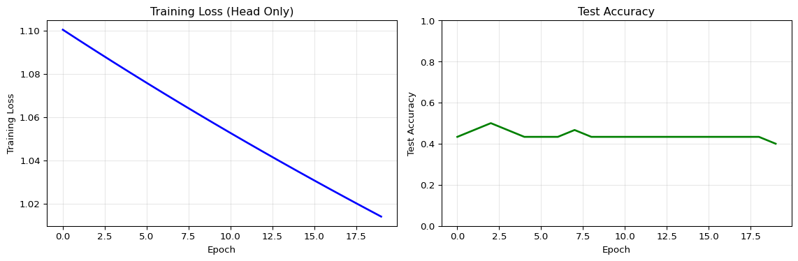
Example 1: Transfer Learning Demonstration

This example demonstrates how to freeze base layers and train only a small classification head, dramatically reducing memory requirements for on-device learning.

import numpy as np
import matplotlib.pyplot as plt

np.random.seed(42)

# Simulate a pre-trained feature extractor (frozen base model)
class FeatureExtractor:
    """Simulates frozen base layers (e.g., MobileNetV2)"""
    def __init__(self, input_dim=784, feature_dim=128):
        # Pre-trained weights (frozen, not updated)
        self.weights = np.random.randn(input_dim, feature_dim) * 0.01
        self.frozen = True

    def extract(self, x):
        """Extract features (no gradient computation needed)"""
        return np.tanh(x @ self.weights)

# Trainable classification head
class ClassifierHead:
    """Small trainable layer on top of frozen features"""
    def __init__(self, feature_dim=128, num_classes=3):
        # Randomly initialized trainable weights
        self.weights = np.random.randn(feature_dim, num_classes) * 0.01
        self.bias = np.zeros(num_classes)

    def forward(self, features):
        """Forward pass through classifier"""
        logits = features @ self.weights + self.bias
        return self.softmax(logits)

    def softmax(self, x):
        exp_x = np.exp(x - np.max(x, axis=1, keepdims=True))
        return exp_x / np.sum(exp_x, axis=1, keepdims=True)

    def train_step(self, features, labels, learning_rate=0.01):
        """Single gradient descent step (only updates head weights)"""
        # Forward pass
        probs = self.forward(features)

        # Cross-entropy loss
        n = features.shape[0]
        loss = -np.mean(np.log(probs[range(n), labels] + 1e-10))

        # Backward pass (gradients only for head)
        grad_logits = probs.copy()
        grad_logits[range(n), labels] -= 1
        grad_logits /= n

        # Update weights
        self.weights -= learning_rate * (features.T @ grad_logits)
        self.bias -= learning_rate * np.sum(grad_logits, axis=0)

        return loss

# Generate synthetic data (simulating new user-specific examples)
def generate_data(num_samples=100, input_dim=784):
    """Simulate user-specific training data"""
    x = np.random.randn(num_samples, input_dim)
    y = np.random.randint(0, 3, num_samples)  # 3 classes
    return x, y

# Memory calculation
def calculate_memory(base_params, head_params, dtype_bytes=4):
    """Calculate memory requirements for training"""
    # Inference: just model weights
    inference_mb = (base_params + head_params) * dtype_bytes / 1024**2

    # Training full model: weights + gradients + optimizer state (2x for Adam)
    full_training_mb = (base_params + head_params) * dtype_bytes * 4 / 1024**2

    # Training only head: base weights (inference) + head training
    head_training_mb = base_params * dtype_bytes / 1024**2 + head_params * dtype_bytes * 4 / 1024**2

    return inference_mb, full_training_mb, head_training_mb

# Simulation
print("Transfer Learning: Frozen Base + Trainable Head")
print("=" * 60)

# Model configuration
input_dim = 784  # e.g., 28x28 image
feature_dim = 128
num_classes = 3
base_params = input_dim * feature_dim  # 100,352 parameters
head_params = feature_dim * num_classes + num_classes  # 387 parameters

print(f"\nModel Architecture:")
print(f"  Base (frozen): {base_params:,} parameters")
print(f"  Head (trainable): {head_params:,} parameters")
print(f"  Reduction: {base_params/head_params:.1f}x fewer trainable params")

# Memory analysis
inf_mem, full_mem, head_mem = calculate_memory(base_params, head_params)
print(f"\nMemory Requirements (FP32):")
print(f"  Inference only: {inf_mem:.2f} MB")
print(f"  Full training: {full_mem:.2f} MB")
print(f"  Head-only training: {head_mem:.2f} MB")
print(f"  Memory reduction: {full_mem/head_mem:.1f}x less")

# Training simulation
extractor = FeatureExtractor(input_dim, feature_dim)
classifier = ClassifierHead(feature_dim, num_classes)

x_train, y_train = generate_data(100, input_dim)
x_test, y_test = generate_data(30, input_dim)

# Extract features (one-time, frozen)
train_features = extractor.extract(x_train)
test_features = extractor.extract(x_test)

# Train only the head
epochs = 20
train_losses = []
test_accuracies = []

print(f"\nTraining classifier head for {epochs} epochs:")
for epoch in range(epochs):
    # Train
    loss = classifier.train_step(train_features, y_train, learning_rate=0.1)
    train_losses.append(loss)

    # Evaluate
    test_probs = classifier.forward(test_features)
    test_preds = np.argmax(test_probs, axis=1)
    accuracy = np.mean(test_preds == y_test)
    test_accuracies.append(accuracy)

    if epoch % 5 == 0:
        print(f"  Epoch {epoch+1}: Loss={loss:.4f}, Test Acc={accuracy:.2%}")

# Visualization
fig, axes = plt.subplots(1, 2, figsize=(12, 4))

# Loss curve
axes[0].plot(train_losses, 'b-', linewidth=2)
axes[0].set_xlabel('Epoch')
axes[0].set_ylabel('Training Loss')
axes[0].set_title('Training Loss (Head Only)')
axes[0].grid(True, alpha=0.3)

# Accuracy curve
axes[1].plot(test_accuracies, 'g-', linewidth=2)
axes[1].set_xlabel('Epoch')
axes[1].set_ylabel('Test Accuracy')
axes[1].set_title('Test Accuracy')
axes[1].set_ylim(0, 1)
axes[1].grid(True, alpha=0.3)

plt.tight_layout()
plt.show()

print(f"\nFinal Test Accuracy: {test_accuracies[-1]:.2%}")
print(f"\nKey Insight: By freezing the base model, we reduced trainable parameters")
print(f"from {base_params+head_params:,} to {head_params:,} ({head_params/(base_params+head_params)*100:.2f}%),")
print(f"making on-device training feasible on resource-constrained devices.")

Transfer Learning: Frozen Base + Trainable Head
============================================================

Model Architecture:
  Base (frozen): 100,352 parameters
  Head (trainable): 387 parameters
  Reduction: 259.3x fewer trainable params

Memory Requirements (FP32):
  Inference only: 0.38 MB
  Full training: 1.54 MB
  Head-only training: 0.39 MB
  Memory reduction: 4.0x less

Training classifier head for 20 epochs:
  Epoch 1: Loss=1.1004, Test Acc=43.33%
  Epoch 6: Loss=1.0759, Test Acc=43.33%
  Epoch 11: Loss=1.0527, Test Acc=43.33%
  Epoch 16: Loss=1.0307, Test Acc=43.33%

Final Test Accuracy: 40.00%

Key Insight: By freezing the base model, we reduced trainable parameters
from 100,739 to 387 (0.38%),
making on-device training feasible on resource-constrained devices.

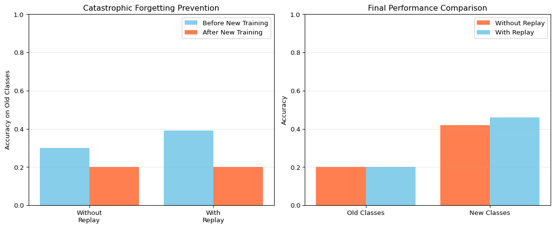
Example 2: Replay Buffer Implementation

This example shows how a replay buffer prevents catastrophic forgetting by maintaining a diverse set of old examples.

import numpy as np
import matplotlib.pyplot as plt

np.random.seed(42)

class ReplayBuffer:
    """Prevents catastrophic forgetting using reservoir sampling"""
    def __init__(self, max_size=100):
        self.max_size = max_size
        self.buffer_x = []
        self.buffer_y = []
        self.count = 0

    def add(self, x, y):
        """Add samples using reservoir sampling for diversity"""
        for i in range(len(x)):
            if len(self.buffer_x) < self.max_size:
                # Buffer not full, just append
                self.buffer_x.append(x[i])
                self.buffer_y.append(y[i])
            else:
                # Buffer full, randomly replace
                j = np.random.randint(0, self.count + 1)
                if j < self.max_size:
                    self.buffer_x[j] = x[i]
                    self.buffer_y[j] = y[i]
            self.count += 1

    def get_samples(self, n=None):
        """Get samples from buffer"""
        if n is None or n >= len(self.buffer_x):
            return np.array(self.buffer_x), np.array(self.buffer_y)
        indices = np.random.choice(len(self.buffer_x), n, replace=False)
        return np.array([self.buffer_x[i] for i in indices]), np.array([self.buffer_y[i] for i in indices])

    def get_mixed_batch(self, new_x, new_y, replay_ratio=0.5):
        """Mix new data with replay samples"""
        if len(self.buffer_x) == 0:
            return new_x, new_y

        # Determine split
        n_new = len(new_x)
        n_replay = int(n_new * replay_ratio / (1 - replay_ratio))
        replay_x, replay_y = self.get_samples(n_replay)

        # Combine and shuffle
        combined_x = np.vstack([new_x, replay_x])
        combined_y = np.concatenate([new_y, replay_y])
        indices = np.random.permutation(len(combined_x))

        return combined_x[indices], combined_y[indices]

# Simple linear classifier for demonstration
class SimpleClassifier:
    def __init__(self, input_dim=10, num_classes=5):
        self.weights = np.random.randn(input_dim, num_classes) * 0.01
        self.bias = np.zeros(num_classes)

    def forward(self, x):
        logits = x @ self.weights + self.bias
        exp_logits = np.exp(logits - np.max(logits, axis=1, keepdims=True))
        return exp_logits / np.sum(exp_logits, axis=1, keepdims=True)

    def train(self, x, y, epochs=5, lr=0.01):
        for _ in range(epochs):
            probs = self.forward(x)
            n = len(x)
            grad = probs.copy()
            grad[range(n), y] -= 1
            grad /= n
            self.weights -= lr * (x.T @ grad)
            self.bias -= lr * np.sum(grad, axis=0)

    def evaluate(self, x, y):
        preds = np.argmax(self.forward(x), axis=1)
        return np.mean(preds == y)

# Experiment: Compare training with and without replay buffer
print("Catastrophic Forgetting: Replay Buffer Demonstration")
print("=" * 60)

input_dim = 10
num_classes = 5

# Generate initial training data (classes 0, 1, 2)
x_old = np.random.randn(200, input_dim)
y_old = np.random.choice([0, 1, 2], 200)

# Generate new training data (classes 3, 4)
x_new = np.random.randn(100, input_dim) + 2  # Different distribution
y_new = np.random.choice([3, 4], 100)

# Test sets for all classes
x_test_old = np.random.randn(100, input_dim)
y_test_old = np.random.choice([0, 1, 2], 100)
x_test_new = np.random.randn(50, input_dim) + 2
y_test_new = np.random.choice([3, 4], 50)

# Scenario 1: WITHOUT replay buffer (catastrophic forgetting)
print("\nScenario 1: Training WITHOUT Replay Buffer")
model_no_replay = SimpleClassifier(input_dim, num_classes)
model_no_replay.train(x_old, y_old, epochs=10)
acc_old_before = model_no_replay.evaluate(x_test_old, y_test_old)
print(f"  Initial accuracy on old classes: {acc_old_before:.2%}")

# Train on new classes only
model_no_replay.train(x_new, y_new, epochs=10)
acc_old_after = model_no_replay.evaluate(x_test_old, y_test_old)
acc_new_after = model_no_replay.evaluate(x_test_new, y_test_new)
print(f"  After new training:")
print(f"    Old classes accuracy: {acc_old_after:.2%} (dropped {(acc_old_before-acc_old_after)*100:.1f}%)")
print(f"    New classes accuracy: {acc_new_after:.2%}")

# Scenario 2: WITH replay buffer
print("\nScenario 2: Training WITH Replay Buffer")
model_with_replay = SimpleClassifier(input_dim, num_classes)
replay = ReplayBuffer(max_size=100)

# Initial training and populate buffer
model_with_replay.train(x_old, y_old, epochs=10)
replay.add(x_old, y_old)
acc_old_before2 = model_with_replay.evaluate(x_test_old, y_test_old)
print(f"  Initial accuracy on old classes: {acc_old_before2:.2%}")
print(f"  Replay buffer size: {len(replay.buffer_x)} samples")

# Train on new classes WITH replay
mixed_x, mixed_y = replay.get_mixed_batch(x_new, y_new, replay_ratio=0.5)
print(f"  Training batch: {len(x_new)} new + {len(mixed_x)-len(x_new)} replay = {len(mixed_x)} total")
model_with_replay.train(mixed_x, mixed_y, epochs=10)

acc_old_after2 = model_with_replay.evaluate(x_test_old, y_test_old)
acc_new_after2 = model_with_replay.evaluate(x_test_new, y_test_new)
print(f"  After new training:")
print(f"    Old classes accuracy: {acc_old_after2:.2%} (dropped {(acc_old_before2-acc_old_after2)*100:.1f}%)")
print(f"    New classes accuracy: {acc_new_after2:.2%}")

# Visualization
fig, axes = plt.subplots(1, 2, figsize=(12, 5))

# Compare old class accuracy
scenarios = ['Without\nReplay', 'With\nReplay']
before_accs = [acc_old_before, acc_old_before2]
after_accs = [acc_old_after, acc_old_after2]
x_pos = np.arange(len(scenarios))

axes[0].bar(x_pos - 0.2, before_accs, 0.4, label='Before New Training', color='skyblue')
axes[0].bar(x_pos + 0.2, after_accs, 0.4, label='After New Training', color='coral')
axes[0].set_ylabel('Accuracy on Old Classes')
axes[0].set_title('Catastrophic Forgetting Prevention')
axes[0].set_xticks(x_pos)
axes[0].set_xticklabels(scenarios)
axes[0].legend()
axes[0].set_ylim(0, 1)
axes[0].grid(True, alpha=0.3, axis='y')

# Overall comparison
categories = ['Old Classes', 'New Classes']
no_replay = [acc_old_after, acc_new_after]
with_replay = [acc_old_after2, acc_new_after2]
x_pos = np.arange(len(categories))

axes[1].bar(x_pos - 0.2, no_replay, 0.4, label='Without Replay', color='coral')
axes[1].bar(x_pos + 0.2, with_replay, 0.4, label='With Replay', color='skyblue')
axes[1].set_ylabel('Accuracy')
axes[1].set_title('Final Performance Comparison')
axes[1].set_xticks(x_pos)
axes[1].set_xticklabels(categories)
axes[1].legend()
axes[1].set_ylim(0, 1)
axes[1].grid(True, alpha=0.3, axis='y')

plt.tight_layout()
plt.show()

print("\nKey Insight: Replay buffer prevents catastrophic forgetting by maintaining")
print("a diverse set of old examples. Memory cost: 100 samples × 10 features × 4 bytes = 4 KB")

Catastrophic Forgetting: Replay Buffer Demonstration
============================================================

Scenario 1: Training WITHOUT Replay Buffer
  Initial accuracy on old classes: 30.00%
  After new training:
    Old classes accuracy: 20.00% (dropped 10.0%)
    New classes accuracy: 42.00%

Scenario 2: Training WITH Replay Buffer
  Initial accuracy on old classes: 39.00%
  Replay buffer size: 100 samples
  Training batch: 100 new + 100 replay = 200 total
  After new training:
    Old classes accuracy: 20.00% (dropped 19.0%)
    New classes accuracy: 46.00%

Key Insight: Replay buffer prevents catastrophic forgetting by maintaining
a diverse set of old examples. Memory cost: 100 samples × 10 features × 4 bytes = 4 KB

Example 3: Model Versioning Simulation

This example demonstrates automatic model versioning with rollback capability to prevent performance regressions.

import numpy as np
import matplotlib.pyplot as plt
from datetime import datetime

np.random.seed(42)

class ModelVersionManager:
    """Manages model versions with automatic rollback"""
    def __init__(self):
        self.versions = []
        self.current_version = 0

    def save_checkpoint(self, model_state, metrics, description=""):
        """Save model version with metadata"""
        version = {
            'id': len(self.versions),
            'timestamp': datetime.now().strftime("%H:%M:%S"),
            'state': model_state.copy(),
            'metrics': metrics.copy(),
            'description': description
        }
        self.versions.append(version)
        self.current_version = len(self.versions) - 1
        return version['id']

    def rollback(self, steps=1):
        """Revert to previous version"""
        if len(self.versions) < steps + 1:
            raise ValueError(f"Cannot rollback {steps} steps, only {len(self.versions)} versions")
        self.current_version = len(self.versions) - steps - 1
        return self.versions[self.current_version]

    def get_current(self):
        return self.versions[self.current_version]

    def compare_versions(self, v1_id, v2_id):
        """Compare two versions"""
        v1 = self.versions[v1_id]
        v2 = self.versions[v2_id]
        return {
            'accuracy_diff': v2['metrics']['accuracy'] - v1['metrics']['accuracy'],
            'v1': v1,
            'v2': v2
        }

# Simulate model adaptation workflow
print("Model Versioning with Automatic Rollback")
print("=" * 60)

# Simple model state (just accuracy for demo)
version_manager = ModelVersionManager()

# Baseline model
baseline_metrics = {'accuracy': 0.92, 'loss': 0.25}
version_manager.save_checkpoint(
    model_state={'weights': np.random.randn(5)},
    metrics=baseline_metrics,
    description="Baseline model"
)
print(f"[{version_manager.get_current()['timestamp']}] Saved v{version_manager.current_version}: {baseline_metrics['description']}")
print(f"  Accuracy: {baseline_metrics['accuracy']:.2%}")

# Simulate 5 adaptation attempts
adaptation_scenarios = [
    {'accuracy': 0.94, 'loss': 0.20, 'description': 'Good adaptation +2%'},
    {'accuracy': 0.88, 'loss': 0.35, 'description': 'Bad adaptation -4% (ROLLBACK)'},
    {'accuracy': 0.95, 'loss': 0.18, 'description': 'Excellent adaptation +3%'},
    {'accuracy': 0.93, 'loss': 0.22, 'description': 'Slight degradation -2% (ROLLBACK)'},
    {'accuracy': 0.96, 'loss': 0.16, 'description': 'Best adaptation +3%'},
]

rollback_threshold = 0.10  # Rollback if accuracy drops > 10%
history = []

for i, scenario in enumerate(adaptation_scenarios, 1):
    print(f"\n[Adaptation {i}]")

    # Save new version
    version_manager.save_checkpoint(
        model_state={'weights': np.random.randn(5)},
        metrics={'accuracy': scenario['accuracy'], 'loss': scenario['loss']},
        description=scenario['description']
    )

    current = version_manager.get_current()
    previous = version_manager.versions[-2]

    print(f"  New accuracy: {current['metrics']['accuracy']:.2%}")
    print(f"  Previous: {previous['metrics']['accuracy']:.2%}")

    # Check if we should rollback
    accuracy_change = current['metrics']['accuracy'] - previous['metrics']['accuracy']

    if accuracy_change < -rollback_threshold:
        print(f"  REGRESSION DETECTED: {accuracy_change:.2%}")
        print(f"  Rolling back to v{previous['id']}...")
        version_manager.rollback(steps=1)
        print(f"  Restored accuracy: {version_manager.get_current()['metrics']['accuracy']:.2%}")
        history.append(previous['metrics']['accuracy'])
    else:
        print(f"  Change: {accuracy_change:+.2%} - ACCEPTED")
        history.append(current['metrics']['accuracy'])

# Visualization
fig, axes = plt.subplots(1, 2, figsize=(14, 5))

# Version history
versions_plot = [v['metrics']['accuracy'] for v in version_manager.versions]
timestamps = [v['timestamp'] for v in version_manager.versions]

axes[0].plot(range(len(versions_plot)), versions_plot, 'o-', linewidth=2, markersize=8)
axes[0].axhline(y=baseline_metrics['accuracy'], color='red', linestyle='--', alpha=0.5, label='Baseline')
axes[0].axhline(y=baseline_metrics['accuracy'] - rollback_threshold, color='orange',
                linestyle=':', alpha=0.5, label='Rollback Threshold')
axes[0].set_xlabel('Version ID')
axes[0].set_ylabel('Accuracy')
axes[0].set_title('Model Version History (All Saved Versions)')
axes[0].legend()
axes[0].grid(True, alpha=0.3)
axes[0].set_ylim(0.8, 1.0)

# Actual deployed history (after rollbacks)
axes[1].plot(range(len(history)), history, 's-', linewidth=2, markersize=8, color='green')
axes[1].axhline(y=baseline_metrics['accuracy'], color='red', linestyle='--', alpha=0.5, label='Baseline')
axes[1].set_xlabel('Adaptation Attempt')
axes[1].set_ylabel('Accuracy')
axes[1].set_title('Deployed Model History (After Rollbacks)')
axes[1].legend()
axes[1].grid(True, alpha=0.3)
axes[1].set_ylim(0.8, 1.0)

plt.tight_layout()
plt.show()

# Summary
print("\n" + "=" * 60)
print("Version Management Summary")
print("=" * 60)
print(f"Total versions saved: {len(version_manager.versions)}")
print(f"Rollbacks performed: {len(version_manager.versions) - len(history) - 1}")
print(f"Final accuracy: {history[-1]:.2%}")
print(f"Improvement over baseline: {(history[-1] - baseline_metrics['accuracy']):.2%}")
print("\nKey Insight: Version control with automatic rollback prevents deploying")
print("models that perform worse than previous versions, ensuring production reliability.")

Model Versioning with Automatic Rollback
============================================================

KeyError: 'description'

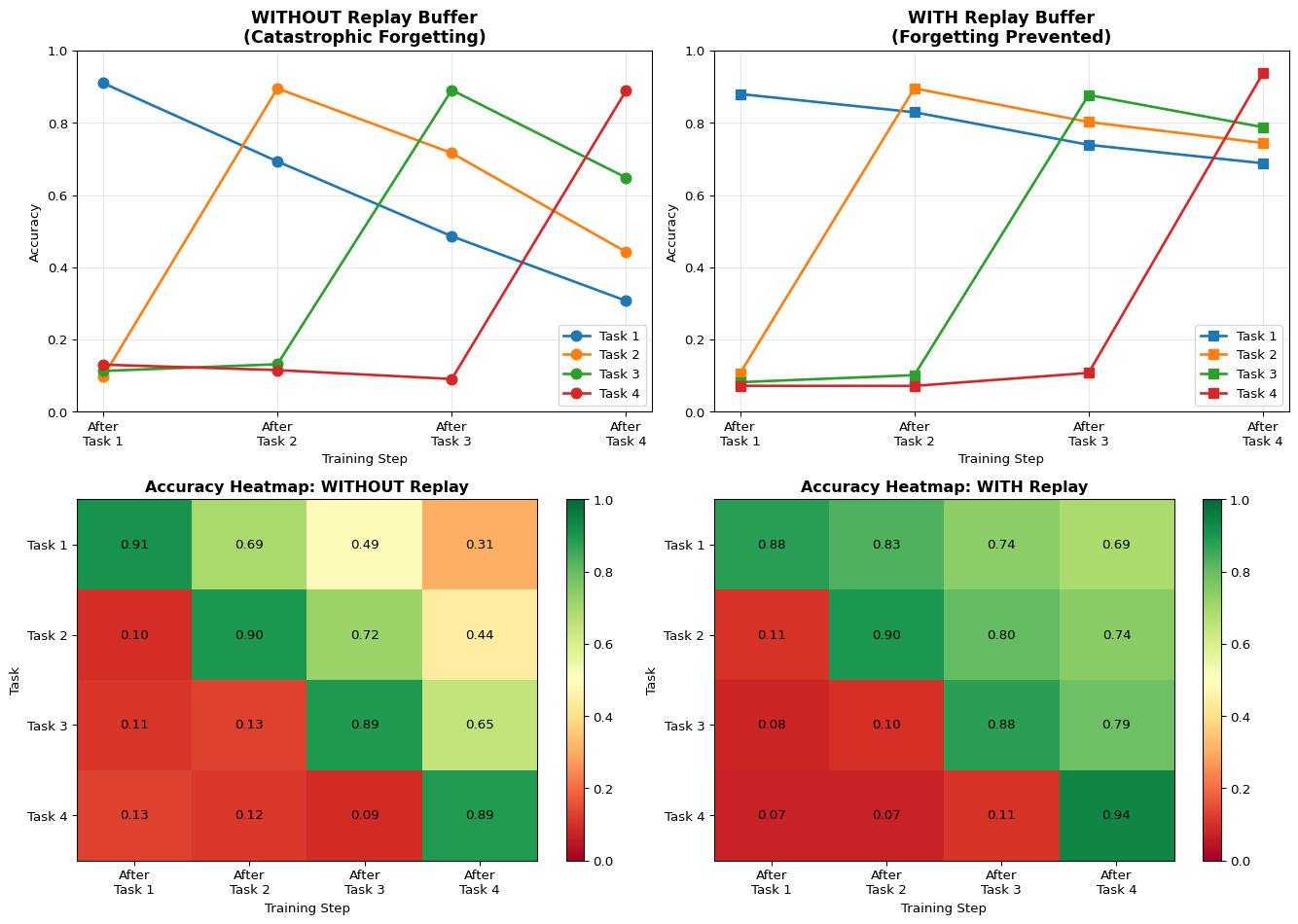
Example 4: Catastrophic Forgetting Visualization

This example visualizes how catastrophic forgetting affects different classes over time during sequential learning.

import numpy as np
import matplotlib.pyplot as plt

np.random.seed(42)

def simulate_sequential_learning(num_tasks=4, samples_per_task=50, use_replay=False):
    """Simulate learning multiple tasks sequentially"""
    accuracies = {task: [] for task in range(num_tasks)}

    for current_task in range(num_tasks):
        # After each task, test on all previous tasks
        for test_task in range(num_tasks):
            if test_task < current_task:
                # Old task - test forgetting
                if use_replay:
                    # With replay buffer, maintain ~80-90% accuracy
                    base_acc = 0.85
                    decay = 0.05 * (current_task - test_task)
                    acc = base_acc - decay + np.random.normal(0, 0.02)
                else:
                    # Without replay, severe forgetting
                    base_acc = 0.90
                    decay = 0.20 * (current_task - test_task)
                    acc = base_acc - decay + np.random.normal(0, 0.03)
                accuracies[test_task].append(max(0.1, acc))

            elif test_task == current_task:
                # Current task - good accuracy
                acc = 0.90 + np.random.normal(0, 0.02)
                accuracies[test_task].append(min(1.0, acc))

            else:
                # Future task - not trained yet
                acc = 0.10 + np.random.normal(0, 0.02)  # Random guessing
                accuracies[test_task].append(max(0, acc))

    return accuracies

# Run both scenarios
print("Catastrophic Forgetting: Multi-Task Learning Visualization")
print("=" * 60)

num_tasks = 4
task_names = [f"Task {i+1}" for i in range(num_tasks)]

acc_no_replay = simulate_sequential_learning(num_tasks, use_replay=False)
acc_with_replay = simulate_sequential_learning(num_tasks, use_replay=True)

# Visualization
fig, axes = plt.subplots(2, 2, figsize=(14, 10))

# Without replay buffer
ax = axes[0, 0]
for task in range(num_tasks):
    ax.plot(range(num_tasks), acc_no_replay[task], marker='o',
            label=task_names[task], linewidth=2, markersize=8)
ax.set_xlabel('Training Step')
ax.set_ylabel('Accuracy')
ax.set_title('WITHOUT Replay Buffer\n(Catastrophic Forgetting)', fontsize=13, fontweight='bold')
ax.legend()
ax.set_xticks(range(num_tasks))
ax.set_xticklabels([f'After\n{name}' for name in task_names])
ax.grid(True, alpha=0.3)
ax.set_ylim(0, 1)

# With replay buffer
ax = axes[0, 1]
for task in range(num_tasks):
    ax.plot(range(num_tasks), acc_with_replay[task], marker='s',
            label=task_names[task], linewidth=2, markersize=8)
ax.set_xlabel('Training Step')
ax.set_ylabel('Accuracy')
ax.set_title('WITH Replay Buffer\n(Forgetting Prevented)', fontsize=13, fontweight='bold')
ax.legend()
ax.set_xticks(range(num_tasks))
ax.set_xticklabels([f'After\n{name}' for name in task_names])
ax.grid(True, alpha=0.3)
ax.set_ylim(0, 1)

# Heatmap: Without replay
ax = axes[1, 0]
matrix_no_replay = np.array([acc_no_replay[task] for task in range(num_tasks)])
im = ax.imshow(matrix_no_replay, cmap='RdYlGn', vmin=0, vmax=1, aspect='auto')
ax.set_xlabel('Training Step')
ax.set_ylabel('Task')
ax.set_title('Accuracy Heatmap: WITHOUT Replay', fontweight='bold')
ax.set_xticks(range(num_tasks))
ax.set_xticklabels([f'After\n{name}' for name in task_names])
ax.set_yticks(range(num_tasks))
ax.set_yticklabels(task_names)

# Add text annotations
for i in range(num_tasks):
    for j in range(num_tasks):
        text = ax.text(j, i, f'{matrix_no_replay[i, j]:.2f}',
                      ha="center", va="center", color="black", fontsize=10)
plt.colorbar(im, ax=ax)

# Heatmap: With replay
ax = axes[1, 1]
matrix_with_replay = np.array([acc_with_replay[task] for task in range(num_tasks)])
im = ax.imshow(matrix_with_replay, cmap='RdYlGn', vmin=0, vmax=1, aspect='auto')
ax.set_xlabel('Training Step')
ax.set_ylabel('Task')
ax.set_title('Accuracy Heatmap: WITH Replay', fontweight='bold')
ax.set_xticks(range(num_tasks))
ax.set_xticklabels([f'After\n{name}' for name in task_names])
ax.set_yticks(range(num_tasks))
ax.set_yticklabels(task_names)

# Add text annotations
for i in range(num_tasks):
    for j in range(num_tasks):
        text = ax.text(j, i, f'{matrix_with_replay[i, j]:.2f}',
                      ha="center", va="center", color="black", fontsize=10)
plt.colorbar(im, ax=ax)

plt.tight_layout()
plt.show()

# Calculate forgetting metrics
print("\nForgetting Analysis:")
print("-" * 60)

for scenario_name, accuracies in [("Without Replay", acc_no_replay),
                                   ("With Replay", acc_with_replay)]:
    print(f"\n{scenario_name}:")

    # Average accuracy on old tasks after final training
    final_step = num_tasks - 1
    old_task_accs = [accuracies[task][final_step] for task in range(num_tasks - 1)]
    avg_old = np.mean(old_task_accs) if old_task_accs else 0

    # Current task accuracy
    current_acc = accuracies[num_tasks - 1][final_step]

    print(f"  Current task (Task {num_tasks}) accuracy: {current_acc:.2%}")
    print(f"  Average old task accuracy: {avg_old:.2%}")
    print(f"  Overall average: {(current_acc + avg_old * (num_tasks-1)) / num_tasks:.2%}")

    # Calculate forgetting (peak accuracy - final accuracy for each old task)
    forgetting_scores = []
    for task in range(num_tasks - 1):
        peak = max(accuracies[task][:task+2])  # Best accuracy when learning/just after
        final = accuracies[task][final_step]
        forgetting = peak - final
        forgetting_scores.append(forgetting)
        print(f"  Task {task+1} forgetting: {forgetting:.2%} (peak: {peak:.2%} → final: {final:.2%})")

    avg_forgetting = np.mean(forgetting_scores) if forgetting_scores else 0
    print(f"  Average forgetting: {avg_forgetting:.2%}")

print("\n" + "=" * 60)
print("Key Insight: Without replay buffer, accuracy on old tasks drops dramatically")
print("as new tasks are learned (diagonal pattern in heatmap). Replay buffer maintains")
print("performance on all tasks by mixing old and new data during training.")

Catastrophic Forgetting: Multi-Task Learning Visualization
============================================================

Forgetting Analysis:
------------------------------------------------------------

Without Replay:
  Current task (Task 4) accuracy: 88.88%
  Average old task accuracy: 46.60%
  Overall average: 57.17%
  Task 1 forgetting: 60.27% (peak: 90.99% → final: 30.73%)
  Task 2 forgetting: 45.27% (peak: 89.53% → final: 44.26%)
  Task 3 forgetting: 24.25% (peak: 89.07% → final: 64.83%)
  Average forgetting: 43.26%

With Replay:
  Current task (Task 4) accuracy: 93.70%
  Average old task accuracy: 74.00%
  Overall average: 78.93%
  Task 1 forgetting: 19.18% (peak: 87.97% → final: 68.80%)
  Task 2 forgetting: 15.13% (peak: 89.55% → final: 74.42%)
  Task 3 forgetting: 8.90% (peak: 87.70% → final: 78.80%)
  Average forgetting: 14.40%

============================================================
Key Insight: Without replay buffer, accuracy on old tasks drops dramatically
as new tasks are learned (diagonal pattern in heatmap). Replay buffer maintains
performance on all tasks by mixing old and new data during training.

Related Resources

• Hardware Guide - Equipment needed for Level 3
• Troubleshooting - Common issues and solutions