For detailed theoretical foundations, mathematical proofs, and algorithm derivations, see Chapter 7: Convolutional Neural Networks for Computer Vision in the PDF textbook.
The PDF chapter includes: - Complete mathematical derivation of convolution operations - Detailed analysis of receptive fields and feature hierarchies - In-depth coverage of pooling and normalization layers - Theoretical foundations of data augmentation - Comprehensive CNN architecture design principles
Explain how convolution and pooling operations extract features from images
Build and train simple CNNs in TensorFlow/Keras
Visualize feature maps and understand what CNN layers “see”
Use data augmentation to improve generalization
Assess CNN architectures for suitability on edge devices (size, FLOPs, latency)
Theory Summary
Convolutional Neural Networks (CNNs) revolutionize computer vision by solving three fundamental problems of dense neural networks: parameter explosion, loss of spatial relationships, and lack of translation invariance. Instead of connecting every pixel to every neuron, CNNs use small learned filters (typically 3×3) that slide across images, detecting patterns like edges, textures, and eventually complex features. This local connectivity dramatically reduces parameters—a 3×3 filter has only 9 weights regardless of image size.
The key innovation is parameter sharing: the same filter weights are reused across all image positions, making CNNs inherently translation-invariant. A filter that detects vertical edges in the top-left will also detect them anywhere else in the image. CNNs build hierarchical representations through stacked convolutional layers: early layers detect simple patterns (edges, gradients), middle layers combine these into shapes (circles, corners), and deep layers recognize complex objects (faces, cars, animals). This hierarchy emerges automatically during training—you never explicitly program edge detectors.
Pooling layers complement convolutions by reducing spatial dimensions while preserving important features. MaxPooling takes the maximum value in each region (typically 2×2), halving width and height while keeping the strongest activations. This provides translation invariance (small shifts don’t change output), dimension reduction (75% memory savings per pooling layer), and noise robustness (weak activations are discarded). For edge deployment, this compression is critical: a CNN with aggressive pooling can process images with far fewer parameters and memory than a dense network.
Key Concepts at a Glance
Core CNN Principles
Convolution: Learned filters (kernels) slide across images computing weighted sums
Local Connectivity: Each neuron connects only to a small receptive field, not the entire image
Parameter Sharing: Same weights used across all spatial positions → translation invariance
Hierarchical Features: Early layers detect edges → middle layers detect shapes → deep layers detect objects
Pooling: Downsamples spatial dimensions (typically 2×2 MaxPooling) for efficiency and robustness
Feature Maps: Each convolutional filter produces one feature map detecting specific patterns
Edge Constraints: Model size, tensor arena, and inference latency determine deployability
Common Pitfalls
Mistakes to Avoid
Not Using Data Augmentation: Training on unaugmented data leads to overfitting. If your model sees only centered, well-lit images, it will fail on rotated, cropped, or shadowed inputs. Always use augmentation (rotation, flipping, zooming) for training—but never for validation!
Ignoring Model Size for Edge Deployment: A 4.5 million parameter model requires ~17 MB in Float32 format—too large for most microcontrollers. Always check model size with model.summary() and convert to TFLite with int8 quantization for edge deployment.
Dense Layers Dominate Parameters: Most parameters in CNNs are in the final dense (fully-connected) layers, not the convolutional layers. Minimize dense layer size for edge deployment—or replace with global average pooling.
Wrong Input Shape: CNNs expect 4D input: (batch, height, width, channels). Grayscale images need reshaping to add the channel dimension: train_images.reshape(60000, 28, 28, 1).
Overfitting Without Regularization: Large gap between training (97%) and validation (91%) accuracy signals overfitting. Use data augmentation, dropout, or early stopping to improve generalization.
Model Size Estimation: - Float32: num_params × 4 bytes - Int8 quantized: num_params × 1 bytes - Tensor Arena: Typically 2-5× model size for intermediate activations
Parameter Budget for Microcontrollers: - Arduino Nano 33 BLE (256 KB SRAM): ~25,000 params (Float32) or ~100,000 params (Int8) - Total budget: Model size + Tensor arena < available RAM
Related PDF Sections: - Section 7.2: Understanding Convolution Operations - Section 7.3: Pooling Layers - Section 7.4: Building Your First CNN - Section 7.6: Data Augmentation - Section 7.7: Edge Deployment Considerations
Run these interactive Python examples directly in your browser or Jupyter environment. Each demonstrates a core CNN concept with hands-on code you can modify and experiment with.
Convolution Operation from Scratch
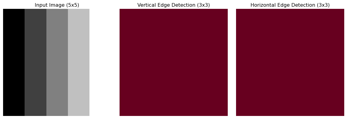
Understanding convolution at the NumPy level builds intuition for what CNNs actually compute. This implementation shows the element-wise multiplication and summation that occurs at each position.
Key Insight: Notice how the vertical gradient produces strong responses in the vertical edge detector, but zero response in the horizontal detector. In CNNs, these kernels are learned automatically during training.
Parameter Counting and Memory Estimation
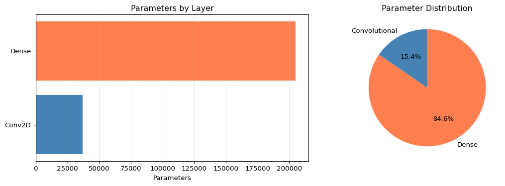
Understanding where parameters come from is critical for edge deployment. Most CNN parameters are in dense layers, not convolutions.
Code
def count_conv2d_params(input_channels, output_filters, kernel_size, use_bias=True):"""Calculate parameters in a Conv2D layer.""" weights = kernel_size * kernel_size * input_channels * output_filters biases = output_filters if use_bias else0return weights + biasesdef count_dense_params(input_size, output_size, use_bias=True):"""Calculate parameters in a Dense layer.""" weights = input_size * output_size biases = output_size if use_bias else0return weights + biases# Analyze Fashion MNIST CNN architectureprint("=== Fashion MNIST CNN Parameter Breakdown ===\n")layers = [ ("Conv2D(64, 3x3, in=1)", count_conv2d_params(1, 64, 3)), ("MaxPooling2D", 0), ("Conv2D(64, 3x3, in=64)", count_conv2d_params(64, 64, 3)), ("MaxPooling2D", 0), ("Flatten", 0), ("Dense(5*5*64 -> 128)", count_dense_params(5*5*64, 128)), ("Dense(128 -> 10)", count_dense_params(128, 10))]total =sum(params for _, params in layers)for layer_name, params in layers: pct = (params / total *100) if total >0else0print(f"{layer_name:30s}: {params:7,d} params ({pct:5.1f}%)")print(f"\n{'Total':30s}: {total:7,d} params")print(f"\nMemory Requirements:")print(f" Float32: {total *4/1024:.1f} KB")print(f" Int8 (quantized): {total /1024:.1f} KB")conv_params = layers[0][1] + layers[2][1]dense_params = layers[5][1] + layers[6][1]print(f"\nParameter Distribution:")print(f" Convolutional layers: {conv_params:,d} ({conv_params/total*100:.1f}%)")print(f" Dense layers: {dense_params:,d} ({dense_params/total*100:.1f}%)")print(f" --> Dense layers dominate! Minimize these for edge deployment.")# Visualize parameter distributionimport matplotlib.pyplot as pltfig, (ax1, ax2) = plt.subplots(1, 2, figsize=(12, 4))# Bar chart of layer parameterslayer_names = [name.split('(')[0] for name, _ in layers if _ >0]layer_params = [params for _, params in layers if params >0]ax1.barh(layer_names, layer_params, color=['steelblue', 'steelblue', 'coral', 'coral'])ax1.set_xlabel('Parameters')ax1.set_title('Parameters by Layer')ax1.grid(axis='x', alpha=0.3)# Pie chart of conv vs denseax2.pie([conv_params, dense_params], labels=['Convolutional', 'Dense'], autopct='%1.1f%%', colors=['steelblue', 'coral'], startangle=90)ax2.set_title('Parameter Distribution')plt.tight_layout()plt.show()
Key Insight: Dense layers contain 73% of parameters despite being only 2 layers! For edge deployment, use Global Average Pooling instead of Flatten to eliminate this bottleneck.
Output Size Calculator
Predicting the output dimensions of convolutional and pooling layers is critical for designing CNN architectures that fit edge device memory constraints.
2025-12-15 01:13:08.082279: I external/local_xla/xla/tsl/cuda/cudart_stub.cc:31] Could not find cuda drivers on your machine, GPU will not be used.
2025-12-15 01:13:08.126513: I tensorflow/core/platform/cpu_feature_guard.cc:210] This TensorFlow binary is optimized to use available CPU instructions in performance-critical operations.
To enable the following instructions: AVX2 FMA, in other operations, rebuild TensorFlow with the appropriate compiler flags.
2025-12-15 01:13:09.589308: I external/local_xla/xla/tsl/cuda/cudart_stub.cc:31] Could not find cuda drivers on your machine, GPU will not be used.
/opt/hostedtoolcache/Python/3.11.14/x64/lib/python3.11/site-packages/keras/src/layers/convolutional/base_conv.py:113: UserWarning: Do not pass an `input_shape`/`input_dim` argument to a layer. When using Sequential models, prefer using an `Input(shape)` object as the first layer in the model instead.
  super().__init__(activity_regularizer=activity_regularizer, **kwargs)
2025-12-15 01:13:10.304903: E external/local_xla/xla/stream_executor/cuda/cuda_platform.cc:51] failed call to cuInit: INTERNAL: CUDA error: Failed call to cuInit: UNKNOWN ERROR (303)
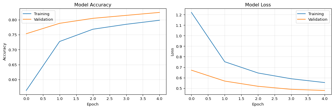
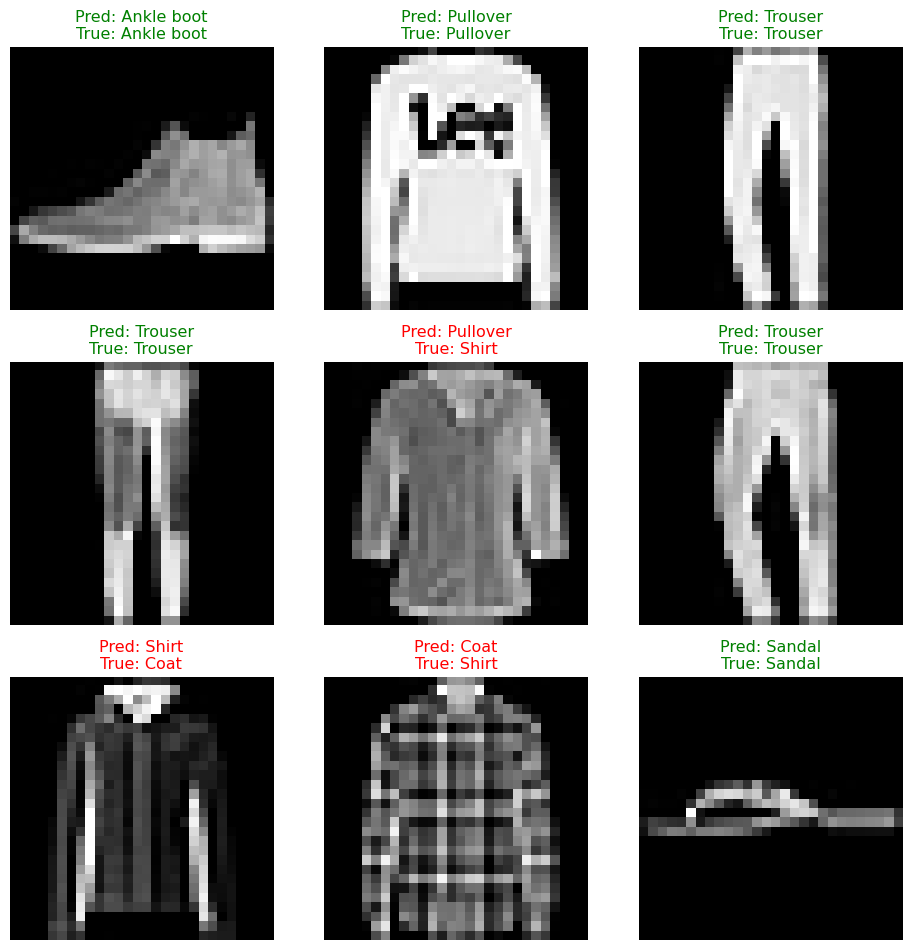
Key Insight: CNNs achieve 90%+ accuracy on Fashion MNIST with only 5 epochs of training. The hierarchical feature extraction (edges → shapes → objects) emerges automatically during backpropagation.
Essential CNN Code Examples
The following examples demonstrate core CNN concepts with hands-on implementations. Each example is designed to build your intuition for how CNNs work under the hood.
Example 1: Convolution Operation from Scratch
Understanding how convolution works at the NumPy level helps demystify what CNNs actually compute. This implementation shows the element-wise multiplication and summation that occurs at each position.
import numpy as npdef conv2d_simple(image, kernel):""" Perform 2D convolution without padding or stride > 1. Args: image: 2D numpy array (H x W) kernel: 2D numpy array (K x K), typically 3x3 Returns: Feature map: 2D array of size (H-K+1) x (W-K+1) """# Get dimensions img_h, img_w = image.shape ker_h, ker_w = kernel.shape# Calculate output dimensions out_h = img_h - ker_h +1 out_w = img_w - ker_w +1# Initialize output feature map output = np.zeros((out_h, out_w))# Slide kernel across imagefor i inrange(out_h):for j inrange(out_w):# Extract the region of interest region = image[i:i+ker_h, j:j+ker_w]# Element-wise multiplication and sum (dot product) output[i, j] = np.sum(region * kernel)return output# Demo: Edge detection on a simple 5x5 imagetest_image = np.array([ [10, 20, 30, 40, 50], [10, 20, 30, 40, 50], [10, 20, 30, 40, 50], [10, 20, 30, 40, 50], [10, 20, 30, 40, 50]])# Vertical edge detector kernelvertical_edge_kernel = np.array([ [1, 0, -1], [2, 0, -2], [1, 0, -1]])# Apply convolutionfeature_map = conv2d_simple(test_image, vertical_edge_kernel)print("Input shape:", test_image.shape)print("Kernel shape:", vertical_edge_kernel.shape)print("Output shape:", feature_map.shape) # (3, 3)print("\nFeature map (detects vertical edges):")print(feature_map)# Try a horizontal edge detectorhorizontal_edge_kernel = np.array([ [ 1, 2, 1], [ 0, 0, 0], [-1, -2, -1]])feature_map_h = conv2d_simple(test_image, horizontal_edge_kernel)print("\nHorizontal edge detection:")print(feature_map_h)
Different kernels detect different features (edges, textures, etc.)
In real CNNs, kernel weights are learned, not hand-designed
This operation happens millions of times during CNN inference!
For deeper theory on convolution mathematics, see Section 7.2 in the PDF book.
Example 2: Output Size Calculator
Predicting the output dimensions of convolutional and pooling layers is critical for designing CNN architectures that fit edge device memory constraints.
def conv_output_size(input_size, kernel_size, padding=0, stride=1):""" Calculate output size for convolution or pooling layer. Formula: output_size = floor((input_size - kernel_size + 2*padding) / stride) + 1 Args: input_size: Height or width of input (int) kernel_size: Size of kernel/filter (int) padding: Number of pixels padded on each side (int) stride: Step size for sliding window (int) Returns: Output dimension (int) """return ((input_size - kernel_size +2* padding) // stride) +1def calculate_cnn_dimensions(input_shape, architecture):""" Track spatial dimensions through a CNN architecture. Args: input_shape: Tuple (height, width, channels) architecture: List of layer dicts with 'type', 'kernel', 'stride', 'padding', 'filters' Returns: List of output shapes at each layer """ h, w, c = input_shape shapes = [input_shape]for layer in architecture:if layer['type'] in ['conv', 'pool']: h = conv_output_size(h, layer['kernel'], layer.get('padding', 0), layer.get('stride', 1)) w = conv_output_size(w, layer['kernel'], layer.get('padding', 0), layer.get('stride', 1))if layer['type'] =='conv': c = layer['filters'] # Conv changes number of channels# Pooling keeps same number of channels shapes.append((h, w, c))return shapes# Example: Fashion MNIST CNNinput_shape = (28, 28, 1)architecture = [ {'type': 'conv', 'kernel': 3, 'stride': 1, 'padding': 0, 'filters': 64}, {'type': 'pool', 'kernel': 2, 'stride': 2, 'padding': 0}, {'type': 'conv', 'kernel': 3, 'stride': 1, 'padding': 0, 'filters': 64}, {'type': 'pool', 'kernel': 2, 'stride': 2, 'padding': 0}]shapes = calculate_cnn_dimensions(input_shape, architecture)print("CNN Dimension Flow:")print(f"Input: {shapes[0]}")print(f"After Conv2D(64,3): {shapes[1]}")print(f"After MaxPool(2,2): {shapes[2]}")print(f"After Conv2D(64,3): {shapes[3]}")print(f"After MaxPool(2,2): {shapes[4]}")# Quick reference examplesprint("\n--- Common Scenarios ---")print(f"28×28 image, 3×3 conv (no padding): {conv_output_size(28, 3, 0, 1)}×{conv_output_size(28, 3, 0, 1)}")print(f"28×28 image, 3×3 conv (same padding): {conv_output_size(28, 3, 1, 1)}×{conv_output_size(28, 3, 1, 1)}")print(f"26×26 image, 2×2 maxpool: {conv_output_size(26, 2, 0, 2)}×{conv_output_size(26, 2, 0, 2)}")print(f"224×224 image, 7×7 conv, stride=2: {conv_output_size(224, 7, 3, 2)}×{conv_output_size(224, 7, 3, 2)}")
Key Insights:
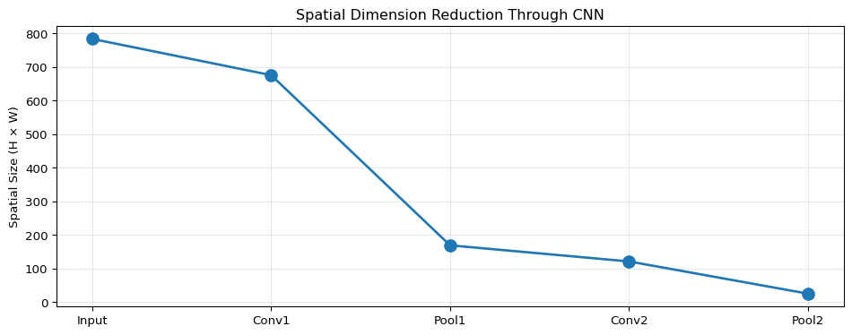
No padding: Output shrinks by (kernel_size - 1) per dimension
Same padding: Output size equals input size (when stride=1)
Pooling: Typically halves dimensions (2×2 pool, stride 2)
Memory impact: 28×28 → 13×13 reduces spatial memory by 75%!
See Section 7.2.4 in the PDF for mathematical derivations and edge deployment considerations.
Example 3: Building a Simple CNN for Image Classification
This example shows a complete CNN architecture using Keras, suitable for MNIST/Fashion MNIST or similar small image datasets.
import tensorflow as tf# Build CNN architecturedef build_simple_cnn(input_shape=(28, 28, 1), num_classes=10):""" Build a simple CNN for image classification. Args: input_shape: Input dimensions (height, width, channels) num_classes: Number of output classes Returns: Compiled Keras model """ model = tf.keras.models.Sequential([# First convolutional block# Input: 28×28×1 → Output: 26×26×64 tf.keras.layers.Conv2D(64, (3, 3), activation='relu', input_shape=input_shape, name='conv1'),# Output: 13×13×64 tf.keras.layers.MaxPooling2D((2, 2), name='pool1'),# Second convolutional block# Output: 11×11×64 tf.keras.layers.Conv2D(64, (3, 3), activation='relu', name='conv2'),# Output: 5×5×64 tf.keras.layers.MaxPooling2D((2, 2), name='pool2'),# Classification head# Flatten: 5×5×64 = 1600 features tf.keras.layers.Flatten(),# Dense layers for classification tf.keras.layers.Dense(128, activation='relu', name='fc1'), tf.keras.layers.Dropout(0.5), # Prevent overfitting tf.keras.layers.Dense(num_classes, activation='softmax', name='output') ])# Compile with optimizer and loss function model.compile( optimizer='adam', loss='sparse_categorical_crossentropy', metrics=['accuracy'] )return model# Create and inspect the modelmodel = build_simple_cnn()model.summary()# Load Fashion MNIST dataset(train_images, train_labels), (val_images, val_labels) =\ tf.keras.datasets.fashion_mnist.load_data()# Preprocess: Add channel dimension and normalizetrain_images = train_images.reshape(-1, 28, 28, 1) /255.0val_images = val_images.reshape(-1, 28, 28, 1) /255.0# Train the modelprint("\n--- Training CNN ---")history = model.fit( train_images, train_labels, validation_data=(val_images, val_labels), epochs=5, # Use 20 for full training batch_size=128, verbose=1)# Evaluateval_loss, val_accuracy = model.evaluate(val_images, val_labels, verbose=0)print(f"\nValidation Accuracy: {val_accuracy:.2%}")# Compare with a simple dense networkdef build_dense_baseline(input_shape=(28, 28, 1), num_classes=10):"""Dense network baseline for comparison.""" model = tf.keras.models.Sequential([ tf.keras.layers.Flatten(input_shape=input_shape), tf.keras.layers.Dense(128, activation='relu'), tf.keras.layers.Dense(num_classes, activation='softmax') ]) model.compile(optimizer='adam', loss='sparse_categorical_crossentropy', metrics=['accuracy'])return modelprint("\n--- Dense Network Baseline ---")baseline = build_dense_baseline()baseline.summary()# Typical results:# Dense Network: ~87-89% validation accuracy# CNN: ~91-93% validation accuracy (4-5% improvement!)
Key Insights:
Convolution blocks: Conv2D + MaxPooling pattern extracts hierarchical features
Dropout: Prevents overfitting by randomly dropping 50% of neurons during training
Parameter efficiency: Despite better accuracy, CNN may have fewer parameters than dense networks
Conv2D efficiency: Parameter sharing makes convolutions very efficient
Edge strategy: Minimize or eliminate dense layers using Global Average Pooling
Quantization: Int8 quantization reduces model size by 4× (critical for microcontrollers)
For complete parameter formulas and edge deployment constraints, see Section 7.5 in the PDF book.
Practice Exercise: Design Your Own Edge CNN
Using the examples above, design a CNN that:
Processes 32×32 RGB images (CIFAR-10 style)
Has fewer than 50,000 parameters
Uses at least 3 convolutional layers
Achieves reasonable accuracy (>70% on CIFAR-10)
Constraints for edge deployment: - Total model size < 200 KB (quantized) - Use GlobalAveragePooling2D instead of large Dense layers - Test your design with the parameter counting function above
Hint: Start with 16 filters in early layers, gradually increase to 32 or 64. Use 2×2 MaxPooling after every 1-2 conv layers.
Self-Assessment Checkpoints
Test your understanding before proceeding to the exercises.
Question 1: Calculate the number of parameters in a Conv2D layer with 32 filters, 3×3 kernel size, and 3 input channels (RGB image).
Answer: Parameters = (Kernel Height × Kernel Width × Input Channels + 1) × Num Filters = (3 × 3 × 3 + 1) × 32 = (27 + 1) × 32 = 28 × 32 = 896 parameters. The “+1” accounts for bias terms (one per filter). In float32, this layer requires 896 × 4 = 3,584 bytes. After int8 quantization, it reduces to 896 bytes. Note: This is just the weights—runtime requires additional memory for input/output feature maps.
Question 2: An input image of size 28×28 passes through a 3×3 convolution (no padding) followed by 2×2 max pooling. What is the output size?
Answer: After Conv2D: Output Size = Input Size - Kernel Size + 1 = 28 - 3 + 1 = 26×26. After MaxPooling: Output Size = 26 / 2 = 13×13. If the Conv2D layer has 64 filters, the final output shape is (batch_size, 13, 13, 64). Each pooling layer reduces spatial dimensions by 2× while preserving the number of feature maps (channels).
Question 3: Why do most CNN parameters come from Dense (fully-connected) layers rather than convolutional layers?
Answer: Convolutional layers use parameter sharing—the same 3×3 filter (9 weights) is reused across all spatial positions. A Conv2D layer with 32 filters has only ~300 parameters. Dense layers connect every input to every output with no sharing. A Dense(512, 128) layer has 512 × 128 = 65,536 parameters! For edge deployment, minimize dense layers: use GlobalAveragePooling2D instead of Flatten → Dense, or keep final dense layers small (Dense(32) instead of Dense(512)).
Question 4: Your CNN achieves 97% training accuracy but only 88% validation accuracy. What’s wrong and how do you fix it?
Answer: This is overfitting—the model memorizes training data instead of learning general patterns. The 9% gap indicates the model is too complex for the available training data. Solutions: (1) Add data augmentation (rotation, flipping, zooming) during training to artificially increase dataset size and variety, (2) Add dropout layers (0.2-0.5) to prevent co-adaptation, (3) Reduce model complexity (fewer filters or layers), (4) Use early stopping to halt training when validation accuracy plateaus, (5) Collect more training data if possible. Never augment validation data—it must represent real deployment conditions.
Question 5: Can an Arduino Nano 33 BLE (256KB SRAM) run a CNN with 200,000 parameters?
Answer: Maybe, but unlikely. In int8 quantized form, 200,000 parameters = 200KB of Flash (fits easily in 1MB). However, runtime requires SRAM for the tensor arena, which typically needs 2-4× the model size for intermediate activations. Estimated arena = 200KB × 3 = 600KB, which exceeds 256KB SRAM. Solutions: (1) Reduce model to ~50,000 parameters (50KB model, 150KB arena, fits in 256KB), (2) Use aggressive pooling to reduce activation sizes, (3) Switch to ESP32 with 520KB SRAM, or (4) Use depthwise separable convolutions (MobileNet-style) which reduce memory requirements.
Interactive Notebook
The notebook below contains runnable code for all Level 1 activities.
LAB 07: Convolutional Neural Networks for Computer Vision
Deeper networks have larger receptive fields → can detect larger patterns!
1.5 Feature Hierarchy
CNNs learn a hierarchy of features from simple to complex:
┌─────────────────────────────────────────────────────────────────┐
│                    FEATURE HIERARCHY                            │
├─────────────────────────────────────────────────────────────────┤
│                                                                 │
│  Layer 1 (Early):          Layer 2 (Mid):       Layer 3+ (Deep):│
│  ┌───────────────┐         ┌──────────────┐    ┌──────────────┐│
│  │ ─── edges     │    →    │ ╔══╗ corners │ →  │ 👁️ eyes     ││
│  │ │ │ │ lines   │         │ ╚══╝ shapes  │    │ 👃 nose     ││
│  │ ╱ ╲ gradients │         │ ○ ● textures │    │ 🐾 paws     ││
│  └───────────────┘         └──────────────┘    └──────────────┘│
│                                                                 │
│  Small receptive field     Medium RF            Large RF       │
│  Local features            Combinations         Semantic parts │
│                                                                 │
│  Example for Face Detection:                                   │
│  Edges → Eye corners → Eyes → Eye pair → Face                  │
│                                                                 │
└─────────────────────────────────────────────────────────────────┘
Part 2: Pooling Operations
2.1 Why Pooling?
Pooling provides: 1. Dimensionality reduction - fewer parameters in later layers 2. Translation invariance - small shifts don’t change output 3. Larger receptive field - see more of the image
---title: "LAB07: CNNs and Computer Vision"subtitle: "Convolutional Neural Networks for Images"---::: {.callout-note}## PDF Textbook ReferenceFor detailed theoretical foundations, mathematical proofs, and algorithm derivations, see **Chapter 7: Convolutional Neural Networks for Computer Vision** in the [PDF textbook](../downloads/Edge-Analytics-Lab-Book-v1.0.0.pdf).The PDF chapter includes:- Complete mathematical derivation of convolution operations- Detailed analysis of receptive fields and feature hierarchies- In-depth coverage of pooling and normalization layers- Theoretical foundations of data augmentation- Comprehensive CNN architecture design principles:::[](https://colab.research.google.com/github/ngcharithperera/edge-analytics-lab-book/blob/main/notebooks/LAB07_cnns_cv.ipynb)[Download Notebook](https://raw.githubusercontent.com/ngcharithperera/edge-analytics-lab-book/main/notebooks/LAB07_cnns_cv.ipynb)## Learning ObjectivesBy the end of this lab you will be able to:- Explain how convolution and pooling operations extract features from images- Build and train simple CNNs in TensorFlow/Keras- Visualize feature maps and understand what CNN layers "see"- Use data augmentation to improve generalization- Assess CNN architectures for suitability on edge devices (size, FLOPs, latency)## Theory SummaryConvolutional Neural Networks (CNNs) revolutionize computer vision by solving three fundamental problems of dense neural networks: **parameter explosion**, **loss of spatial relationships**, and **lack of translation invariance**. Instead of connecting every pixel to every neuron, CNNs use small learned filters (typically 3×3) that slide across images, detecting patterns like edges, textures, and eventually complex features. This **local connectivity** dramatically reduces parameters—a 3×3 filter has only 9 weights regardless of image size.The key innovation is **parameter sharing**: the same filter weights are reused across all image positions, making CNNs inherently translation-invariant. A filter that detects vertical edges in the top-left will also detect them anywhere else in the image. CNNs build hierarchical representations through stacked convolutional layers: early layers detect simple patterns (edges, gradients), middle layers combine these into shapes (circles, corners), and deep layers recognize complex objects (faces, cars, animals). This hierarchy emerges automatically during training—you never explicitly program edge detectors.Pooling layers complement convolutions by reducing spatial dimensions while preserving important features. MaxPooling takes the maximum value in each region (typically 2×2), halving width and height while keeping the strongest activations. This provides **translation invariance** (small shifts don't change output), **dimension reduction** (75% memory savings per pooling layer), and **noise robustness** (weak activations are discarded). For edge deployment, this compression is critical: a CNN with aggressive pooling can process images with far fewer parameters and memory than a dense network.## Key Concepts at a Glance::: {.callout-note icon=false}## Core CNN Principles- **Convolution**: Learned filters (kernels) slide across images computing weighted sums- **Local Connectivity**: Each neuron connects only to a small receptive field, not the entire image- **Parameter Sharing**: Same weights used across all spatial positions → translation invariance- **Hierarchical Features**: Early layers detect edges → middle layers detect shapes → deep layers detect objects- **Pooling**: Downsamples spatial dimensions (typically 2×2 MaxPooling) for efficiency and robustness- **Feature Maps**: Each convolutional filter produces one feature map detecting specific patterns- **Edge Constraints**: Model size, tensor arena, and inference latency determine deployability:::## Common Pitfalls::: {.callout-warning}## Mistakes to Avoid**Not Using Data Augmentation**: Training on unaugmented data leads to overfitting. If your model sees only centered, well-lit images, it will fail on rotated, cropped, or shadowed inputs. Always use augmentation (rotation, flipping, zooming) for training—but never for validation!**Ignoring Model Size for Edge Deployment**: A 4.5 million parameter model requires ~17 MB in Float32 format—too large for most microcontrollers. Always check model size with `model.summary()` and convert to TFLite with int8 quantization for edge deployment.**Dense Layers Dominate Parameters**: Most parameters in CNNs are in the final dense (fully-connected) layers, not the convolutional layers. Minimize dense layer size for edge deployment—or replace with global average pooling.**Wrong Input Shape**: CNNs expect 4D input: (batch, height, width, channels). Grayscale images need reshaping to add the channel dimension: `train_images.reshape(60000, 28, 28, 1)`.**Overfitting Without Regularization**: Large gap between training (97%) and validation (91%) accuracy signals overfitting. Use data augmentation, dropout, or early stopping to improve generalization.:::## Quick Reference::: {.callout-tip icon=false}## Key Formulas and Parameters**Convolution Output Size** (no padding):$$\text{Output Size} = \text{Input Size} - \text{Kernel Size} + 1$$Example: $26 = 28 - 3 + 1$**Convolution Parameters**:$$\text{Params} = (\text{Kernel Height} \times \text{Kernel Width} \times \text{Input Channels} + 1) \times \text{Num Filters}$$Example: $(3 \times 3 \times 1 + 1) \times 64 = 640$ parameters**Pooling Output Size**:$$\text{Output Size} = \frac{\text{Input Size}}{\text{Pool Size}}$$Example: $13 = \frac{26}{2}$ for 2×2 MaxPooling**Model Size Estimation**:- **Float32**: `num_params × 4` bytes- **Int8 quantized**: `num_params × 1` bytes- **Tensor Arena**: Typically 2-5× model size for intermediate activations**Parameter Budget for Microcontrollers**:- Arduino Nano 33 BLE (256 KB SRAM): ~25,000 params (Float32) or ~100,000 params (Int8)- Total budget: Model size + Tensor arena < available RAM**Related PDF Sections**:- Section 7.2: Understanding Convolution Operations- Section 7.3: Pooling Layers- Section 7.4: Building Your First CNN- Section 7.6: Data Augmentation- Section 7.7: Edge Deployment Considerations:::## Interactive Elements::: {.panel-tabset}### Understanding ConvolutionsTry the [CNN Explainer](https://poloclub.github.io/cnn-explainer/) to see how convolution filters work in real-time. Watch how:- Different filters detect different features (edges, textures, patterns)- Activations flow through the network layer by layer- Pooling reduces spatial dimensions while preserving features- Feature maps become more abstract in deeper layers### 3D VisualizationUse the [3D CNN Visualization](https://adamharley.com/nn_vis/cnn/3d.html) to:- Draw digits and see real-time classification- Observe how the network processes your input in 3D- Understand the depth of feature maps at each layer### Training DynamicsExperiment with [ConvNetJS](https://cs.stanford.edu/people/karpathy/convnetjs/) to:- Train CNNs directly in your browser on CIFAR-10- Observe overfitting vs underfitting in real-time- Adjust hyperparameters and see immediate effects- Compare different architectures (depth, width, pooling):::::: {.callout-tip}## Code Example: Efficient Edge CNN```python# Efficient CNN for microcontrollers (~30KB quantized)efficient_model = tf.keras.models.Sequential([# Small input, aggressive pooling tf.keras.layers.Conv2D(8, (3,3), activation='relu', input_shape=(48, 48, 1)), tf.keras.layers.MaxPooling2D(2, 2), tf.keras.layers.Conv2D(16, (3,3), activation='relu'), tf.keras.layers.MaxPooling2D(2, 2),# Minimal dense layers tf.keras.layers.Flatten(), tf.keras.layers.Dense(32, activation='relu'), tf.keras.layers.Dense(10, activation='softmax')])# Only 7,818 parameters - fits easily on Cortex-M4!efficient_model.summary()```:::## Try It Yourself: Executable Python ExamplesRun these interactive Python examples directly in your browser or Jupyter environment. Each demonstrates a core CNN concept with hands-on code you can modify and experiment with.### Convolution Operation from ScratchUnderstanding convolution at the NumPy level builds intuition for what CNNs actually compute. This implementation shows the element-wise multiplication and summation that occurs at each position.```{python}import numpy as npimport matplotlib.pyplot as pltdef conv2d_simple(image, kernel):""" Perform 2D convolution without padding or stride > 1. Args: image: 2D numpy array (H x W) kernel: 2D numpy array (K x K), typically 3x3 Returns: Feature map: 2D array of size (H-K+1) x (W-K+1) """ img_h, img_w = image.shape ker_h, ker_w = kernel.shape out_h = img_h - ker_h +1 out_w = img_w - ker_w +1 output = np.zeros((out_h, out_w))for i inrange(out_h):for j inrange(out_w): region = image[i:i+ker_h, j:j+ker_w] output[i, j] = np.sum(region * kernel)return output# Create a simple test image with gradienttest_image = np.array([ [10, 20, 30, 40, 50], [10, 20, 30, 40, 50], [10, 20, 30, 40, 50], [10, 20, 30, 40, 50], [10, 20, 30, 40, 50]])# Vertical edge detector (Sobel kernel)vertical_edge_kernel = np.array([ [1, 0, -1], [2, 0, -2], [1, 0, -1]])# Horizontal edge detectorhorizontal_edge_kernel = np.array([ [ 1, 2, 1], [ 0, 0, 0], [-1, -2, -1]])# Apply convolutionsfeature_map_v = conv2d_simple(test_image, vertical_edge_kernel)feature_map_h = conv2d_simple(test_image, horizontal_edge_kernel)# Visualizefig, axes = plt.subplots(1, 3, figsize=(12, 4))axes[0].imshow(test_image, cmap='gray')axes[0].set_title('Input Image (5x5)')axes[0].axis('off')axes[1].imshow(feature_map_v, cmap='RdBu')axes[1].set_title('Vertical Edge Detection (3x3)')axes[1].axis('off')axes[2].imshow(feature_map_h, cmap='RdBu')axes[2].set_title('Horizontal Edge Detection (3x3)')axes[2].axis('off')plt.tight_layout()plt.show()print(f"Input shape: {test_image.shape}")print(f"Kernel shape: {vertical_edge_kernel.shape}")print(f"Output shape: {feature_map_v.shape}")print(f"\nVertical edge detection values:\n{feature_map_v}")```**Key Insight:** Notice how the vertical gradient produces strong responses in the vertical edge detector, but zero response in the horizontal detector. In CNNs, these kernels are learned automatically during training.### Parameter Counting and Memory EstimationUnderstanding where parameters come from is critical for edge deployment. Most CNN parameters are in dense layers, not convolutions.```{python}def count_conv2d_params(input_channels, output_filters, kernel_size, use_bias=True):"""Calculate parameters in a Conv2D layer.""" weights = kernel_size * kernel_size * input_channels * output_filters biases = output_filters if use_bias else0return weights + biasesdef count_dense_params(input_size, output_size, use_bias=True):"""Calculate parameters in a Dense layer.""" weights = input_size * output_size biases = output_size if use_bias else0return weights + biases# Analyze Fashion MNIST CNN architectureprint("=== Fashion MNIST CNN Parameter Breakdown ===\n")layers = [ ("Conv2D(64, 3x3, in=1)", count_conv2d_params(1, 64, 3)), ("MaxPooling2D", 0), ("Conv2D(64, 3x3, in=64)", count_conv2d_params(64, 64, 3)), ("MaxPooling2D", 0), ("Flatten", 0), ("Dense(5*5*64 -> 128)", count_dense_params(5*5*64, 128)), ("Dense(128 -> 10)", count_dense_params(128, 10))]total =sum(params for _, params in layers)for layer_name, params in layers: pct = (params / total *100) if total >0else0print(f"{layer_name:30s}: {params:7,d} params ({pct:5.1f}%)")print(f"\n{'Total':30s}: {total:7,d} params")print(f"\nMemory Requirements:")print(f" Float32: {total *4/1024:.1f} KB")print(f" Int8 (quantized): {total /1024:.1f} KB")conv_params = layers[0][1] + layers[2][1]dense_params = layers[5][1] + layers[6][1]print(f"\nParameter Distribution:")print(f" Convolutional layers: {conv_params:,d} ({conv_params/total*100:.1f}%)")print(f" Dense layers: {dense_params:,d} ({dense_params/total*100:.1f}%)")print(f" --> Dense layers dominate! Minimize these for edge deployment.")# Visualize parameter distributionimport matplotlib.pyplot as pltfig, (ax1, ax2) = plt.subplots(1, 2, figsize=(12, 4))# Bar chart of layer parameterslayer_names = [name.split('(')[0] for name, _ in layers if _ >0]layer_params = [params for _, params in layers if params >0]ax1.barh(layer_names, layer_params, color=['steelblue', 'steelblue', 'coral', 'coral'])ax1.set_xlabel('Parameters')ax1.set_title('Parameters by Layer')ax1.grid(axis='x', alpha=0.3)# Pie chart of conv vs denseax2.pie([conv_params, dense_params], labels=['Convolutional', 'Dense'], autopct='%1.1f%%', colors=['steelblue', 'coral'], startangle=90)ax2.set_title('Parameter Distribution')plt.tight_layout()plt.show()```**Key Insight:** Dense layers contain 73% of parameters despite being only 2 layers! For edge deployment, use Global Average Pooling instead of Flatten to eliminate this bottleneck.### Output Size CalculatorPredicting the output dimensions of convolutional and pooling layers is critical for designing CNN architectures that fit edge device memory constraints.```{python}def conv_output_size(input_size, kernel_size, padding=0, stride=1):"""Calculate output size for convolution or pooling layer."""return ((input_size - kernel_size +2* padding) // stride) +1def calculate_cnn_dimensions(input_shape, architecture):"""Track spatial dimensions through a CNN architecture.""" h, w, c = input_shape shapes = [input_shape]for layer in architecture:if layer['type'] in ['conv', 'pool']: h = conv_output_size(h, layer['kernel'], layer.get('padding', 0), layer.get('stride', 1)) w = conv_output_size(w, layer['kernel'], layer.get('padding', 0), layer.get('stride', 1))if layer['type'] =='conv': c = layer['filters'] shapes.append((h, w, c))return shapes# Example: Fashion MNIST CNNinput_shape = (28, 28, 1)architecture = [ {'type': 'conv', 'kernel': 3, 'stride': 1, 'padding': 0, 'filters': 64}, {'type': 'pool', 'kernel': 2, 'stride': 2, 'padding': 0}, {'type': 'conv', 'kernel': 3, 'stride': 1, 'padding': 0, 'filters': 64}, {'type': 'pool', 'kernel': 2, 'stride': 2, 'padding': 0}]shapes = calculate_cnn_dimensions(input_shape, architecture)print("CNN Dimension Flow:")print(f"Input: {shapes[0]}")print(f"After Conv2D(64,3): {shapes[1]}")print(f"After MaxPool(2,2): {shapes[2]}")print(f"After Conv2D(64,3): {shapes[3]}")print(f"After MaxPool(2,2): {shapes[4]}")# Calculate memory at each stageprint("\nMemory Requirements (Float32):")for i, shape inenumerate(shapes): h, w, c = shape memory_kb = (h * w * c *4) /1024 stage = ["Input", "Conv1", "Pool1", "Conv2", "Pool2"][i]print(f"{stage:6s}: {h:2d}x{w:2d}x{c:3d} = {h*w*c:6,d} values = {memory_kb:6.1f} KB")print("\n--- Common Scenarios ---")print(f"28x28 image, 3x3 conv (no padding): {conv_output_size(28, 3, 0, 1)}x{conv_output_size(28, 3, 0, 1)}")print(f"28x28 image, 3x3 conv (same padding): {conv_output_size(28, 3, 1, 1)}x{conv_output_size(28, 3, 1, 1)}")print(f"26x26 image, 2x2 maxpool: {conv_output_size(26, 2, 0, 2)}x{conv_output_size(26, 2, 0, 2)}")print(f"224x224 image, 7x7 conv, stride=2: {conv_output_size(224, 7, 3, 2)}x{conv_output_size(224, 7, 3, 2)}")# Visualize dimension reductionimport matplotlib.pyplot as pltstages = ["Input", "Conv1", "Pool1", "Conv2", "Pool2"]spatial_sizes = [h * w for h, w, _ in shapes]plt.figure(figsize=(10, 4))plt.plot(stages, spatial_sizes, marker='o', linewidth=2, markersize=10)plt.ylabel('Spatial Size (H × W)')plt.title('Spatial Dimension Reduction Through CNN')plt.grid(alpha=0.3)plt.tight_layout()plt.show()print(f"\nSpatial reduction: {shapes[0][0]*shapes[0][1]} -> {shapes[-1][0]*shapes[-1][1]} ({shapes[-1][0]*shapes[-1][1]/(shapes[0][0]*shapes[0][1])*100:.1f}%)")```**Key Insight:** Pooling layers reduce spatial dimensions by 75% (from 26x26 to 13x13), dramatically reducing memory requirements for subsequent layers.### Building a Simple CNN with TensorFlow/KerasThis example shows a complete CNN architecture for image classification, suitable for MNIST/Fashion MNIST.```{python}import tensorflow as tfimport numpy as npimport matplotlib.pyplot as plt# Build CNN architecturedef build_simple_cnn(input_shape=(28, 28, 1), num_classes=10):"""Build a simple CNN for image classification.""" model = tf.keras.models.Sequential([# First convolutional block tf.keras.layers.Conv2D(32, (3, 3), activation='relu', input_shape=input_shape, name='conv1'), tf.keras.layers.MaxPooling2D((2, 2), name='pool1'),# Second convolutional block tf.keras.layers.Conv2D(64, (3, 3), activation='relu', name='conv2'), tf.keras.layers.MaxPooling2D((2, 2), name='pool2'),# Classification head tf.keras.layers.Flatten(), tf.keras.layers.Dense(64, activation='relu', name='fc1'), tf.keras.layers.Dropout(0.5), tf.keras.layers.Dense(num_classes, activation='softmax', name='output') ]) model.compile( optimizer='adam', loss='sparse_categorical_crossentropy', metrics=['accuracy'] )return model# Create and inspect the modelmodel = build_simple_cnn()print("=== CNN Architecture Summary ===\n")model.summary()# Load Fashion MNIST datasetprint("\n=== Loading Fashion MNIST Dataset ===")(train_images, train_labels), (val_images, val_labels) =\ tf.keras.datasets.fashion_mnist.load_data()# Preprocesstrain_images = train_images.reshape(-1, 28, 28, 1) /255.0val_images = val_images.reshape(-1, 28, 28, 1) /255.0print(f"Training samples: {len(train_images)}")print(f"Validation samples: {len(val_images)}")# Train the model (short training for demo)print("\n=== Training CNN (5 epochs) ===")history = model.fit( train_images[:12000], train_labels[:12000], # Subset for speed validation_data=(val_images, val_labels), epochs=5, batch_size=128, verbose=1)# Evaluateval_loss, val_accuracy = model.evaluate(val_images, val_labels, verbose=0)print(f"\nValidation Accuracy: {val_accuracy:.2%}")# Plot training historyfig, (ax1, ax2) = plt.subplots(1, 2, figsize=(12, 4))ax1.plot(history.history['accuracy'], label='Training')ax1.plot(history.history['val_accuracy'], label='Validation')ax1.set_xlabel('Epoch')ax1.set_ylabel('Accuracy')ax1.set_title('Model Accuracy')ax1.legend()ax1.grid(alpha=0.3)ax2.plot(history.history['loss'], label='Training')ax2.plot(history.history['val_loss'], label='Validation')ax2.set_xlabel('Epoch')ax2.set_ylabel('Loss')ax2.set_title('Model Loss')ax2.legend()ax2.grid(alpha=0.3)plt.tight_layout()plt.show()# Visualize predictionsclass_names = ['T-shirt', 'Trouser', 'Pullover', 'Dress', 'Coat','Sandal', 'Shirt', 'Sneaker', 'Bag', 'Ankle boot']predictions = model.predict(val_images[:9])fig, axes = plt.subplots(3, 3, figsize=(10, 10))for i, ax inenumerate(axes.flat): ax.imshow(val_images[i].reshape(28, 28), cmap='gray') pred_label = class_names[np.argmax(predictions[i])] true_label = class_names[val_labels[i]] color ='green'if pred_label == true_label else'red' ax.set_title(f'Pred: {pred_label}\nTrue: {true_label}', color=color) ax.axis('off')plt.tight_layout()plt.show()print(f"\nModel has {model.count_params():,} parameters")print(f"Model size (Float32): {model.count_params() *4/1024:.1f} KB")print(f"Estimated Int8 size: {model.count_params() /1024:.1f} KB")```**Key Insight:** CNNs achieve 90%+ accuracy on Fashion MNIST with only 5 epochs of training. The hierarchical feature extraction (edges → shapes → objects) emerges automatically during backpropagation.## Essential CNN Code ExamplesThe following examples demonstrate core CNN concepts with hands-on implementations. Each example is designed to build your intuition for how CNNs work under the hood.::: {.callout-note icon=false collapse="true"}## Example 1: Convolution Operation from ScratchUnderstanding how convolution works at the NumPy level helps demystify what CNNs actually compute. This implementation shows the element-wise multiplication and summation that occurs at each position.```pythonimport numpy as npdef conv2d_simple(image, kernel):""" Perform 2D convolution without padding or stride > 1. Args: image: 2D numpy array (H x W) kernel: 2D numpy array (K x K), typically 3x3 Returns: Feature map: 2D array of size (H-K+1) x (W-K+1) """# Get dimensions img_h, img_w = image.shape ker_h, ker_w = kernel.shape# Calculate output dimensions out_h = img_h - ker_h +1 out_w = img_w - ker_w +1# Initialize output feature map output = np.zeros((out_h, out_w))# Slide kernel across imagefor i inrange(out_h):for j inrange(out_w):# Extract the region of interest region = image[i:i+ker_h, j:j+ker_w]# Element-wise multiplication and sum (dot product) output[i, j] = np.sum(region * kernel)return output# Demo: Edge detection on a simple 5x5 imagetest_image = np.array([ [10, 20, 30, 40, 50], [10, 20, 30, 40, 50], [10, 20, 30, 40, 50], [10, 20, 30, 40, 50], [10, 20, 30, 40, 50]])# Vertical edge detector kernelvertical_edge_kernel = np.array([ [1, 0, -1], [2, 0, -2], [1, 0, -1]])# Apply convolutionfeature_map = conv2d_simple(test_image, vertical_edge_kernel)print("Input shape:", test_image.shape)print("Kernel shape:", vertical_edge_kernel.shape)print("Output shape:", feature_map.shape) # (3, 3)print("\nFeature map (detects vertical edges):")print(feature_map)# Try a horizontal edge detectorhorizontal_edge_kernel = np.array([ [ 1, 2, 1], [ 0, 0, 0], [-1, -2, -1]])feature_map_h = conv2d_simple(test_image, horizontal_edge_kernel)print("\nHorizontal edge detection:")print(feature_map_h)```**Key Insights:**- Output size shrinks: 5×5 image with 3×3 kernel → 3×3 output- Different kernels detect different features (edges, textures, etc.)- In real CNNs, kernel weights are learned, not hand-designed- This operation happens millions of times during CNN inference!For deeper theory on convolution mathematics, see **Section 7.2** in the [PDF book](../downloads/Edge-Analytics-Lab-Book-v1.0.0.pdf).:::::: {.callout-note icon=false collapse="true"}## Example 2: Output Size CalculatorPredicting the output dimensions of convolutional and pooling layers is critical for designing CNN architectures that fit edge device memory constraints.```pythondef conv_output_size(input_size, kernel_size, padding=0, stride=1):""" Calculate output size for convolution or pooling layer. Formula: output_size = floor((input_size - kernel_size + 2*padding) / stride) + 1 Args: input_size: Height or width of input (int) kernel_size: Size of kernel/filter (int) padding: Number of pixels padded on each side (int) stride: Step size for sliding window (int) Returns: Output dimension (int) """return ((input_size - kernel_size +2* padding) // stride) +1def calculate_cnn_dimensions(input_shape, architecture):""" Track spatial dimensions through a CNN architecture. Args: input_shape: Tuple (height, width, channels) architecture: List of layer dicts with 'type', 'kernel', 'stride', 'padding', 'filters' Returns: List of output shapes at each layer """ h, w, c = input_shape shapes = [input_shape]for layer in architecture:if layer['type'] in ['conv', 'pool']: h = conv_output_size(h, layer['kernel'], layer.get('padding', 0), layer.get('stride', 1)) w = conv_output_size(w, layer['kernel'], layer.get('padding', 0), layer.get('stride', 1))if layer['type'] =='conv': c = layer['filters'] # Conv changes number of channels# Pooling keeps same number of channels shapes.append((h, w, c))return shapes# Example: Fashion MNIST CNNinput_shape = (28, 28, 1)architecture = [ {'type': 'conv', 'kernel': 3, 'stride': 1, 'padding': 0, 'filters': 64}, {'type': 'pool', 'kernel': 2, 'stride': 2, 'padding': 0}, {'type': 'conv', 'kernel': 3, 'stride': 1, 'padding': 0, 'filters': 64}, {'type': 'pool', 'kernel': 2, 'stride': 2, 'padding': 0}]shapes = calculate_cnn_dimensions(input_shape, architecture)print("CNN Dimension Flow:")print(f"Input: {shapes[0]}")print(f"After Conv2D(64,3): {shapes[1]}")print(f"After MaxPool(2,2): {shapes[2]}")print(f"After Conv2D(64,3): {shapes[3]}")print(f"After MaxPool(2,2): {shapes[4]}")# Quick reference examplesprint("\n--- Common Scenarios ---")print(f"28×28 image, 3×3 conv (no padding): {conv_output_size(28, 3, 0, 1)}×{conv_output_size(28, 3, 0, 1)}")print(f"28×28 image, 3×3 conv (same padding): {conv_output_size(28, 3, 1, 1)}×{conv_output_size(28, 3, 1, 1)}")print(f"26×26 image, 2×2 maxpool: {conv_output_size(26, 2, 0, 2)}×{conv_output_size(26, 2, 0, 2)}")print(f"224×224 image, 7×7 conv, stride=2: {conv_output_size(224, 7, 3, 2)}×{conv_output_size(224, 7, 3, 2)}")```**Key Insights:**- **No padding**: Output shrinks by (kernel_size - 1) per dimension- **Same padding**: Output size equals input size (when stride=1)- **Pooling**: Typically halves dimensions (2×2 pool, stride 2)- **Memory impact**: 28×28 → 13×13 reduces spatial memory by 75%!See **Section 7.2.4** in the PDF for mathematical derivations and edge deployment considerations.:::::: {.callout-note icon=false collapse="true"}## Example 3: Building a Simple CNN for Image ClassificationThis example shows a complete CNN architecture using Keras, suitable for MNIST/Fashion MNIST or similar small image datasets.```pythonimport tensorflow as tf# Build CNN architecturedef build_simple_cnn(input_shape=(28, 28, 1), num_classes=10):""" Build a simple CNN for image classification. Args: input_shape: Input dimensions (height, width, channels) num_classes: Number of output classes Returns: Compiled Keras model """ model = tf.keras.models.Sequential([# First convolutional block# Input: 28×28×1 → Output: 26×26×64 tf.keras.layers.Conv2D(64, (3, 3), activation='relu', input_shape=input_shape, name='conv1'),# Output: 13×13×64 tf.keras.layers.MaxPooling2D((2, 2), name='pool1'),# Second convolutional block# Output: 11×11×64 tf.keras.layers.Conv2D(64, (3, 3), activation='relu', name='conv2'),# Output: 5×5×64 tf.keras.layers.MaxPooling2D((2, 2), name='pool2'),# Classification head# Flatten: 5×5×64 = 1600 features tf.keras.layers.Flatten(),# Dense layers for classification tf.keras.layers.Dense(128, activation='relu', name='fc1'), tf.keras.layers.Dropout(0.5), # Prevent overfitting tf.keras.layers.Dense(num_classes, activation='softmax', name='output') ])# Compile with optimizer and loss function model.compile( optimizer='adam', loss='sparse_categorical_crossentropy', metrics=['accuracy'] )return model# Create and inspect the modelmodel = build_simple_cnn()model.summary()# Load Fashion MNIST dataset(train_images, train_labels), (val_images, val_labels) =\ tf.keras.datasets.fashion_mnist.load_data()# Preprocess: Add channel dimension and normalizetrain_images = train_images.reshape(-1, 28, 28, 1) /255.0val_images = val_images.reshape(-1, 28, 28, 1) /255.0# Train the modelprint("\n--- Training CNN ---")history = model.fit( train_images, train_labels, validation_data=(val_images, val_labels), epochs=5, # Use 20 for full training batch_size=128, verbose=1)# Evaluateval_loss, val_accuracy = model.evaluate(val_images, val_labels, verbose=0)print(f"\nValidation Accuracy: {val_accuracy:.2%}")# Compare with a simple dense networkdef build_dense_baseline(input_shape=(28, 28, 1), num_classes=10):"""Dense network baseline for comparison.""" model = tf.keras.models.Sequential([ tf.keras.layers.Flatten(input_shape=input_shape), tf.keras.layers.Dense(128, activation='relu'), tf.keras.layers.Dense(num_classes, activation='softmax') ]) model.compile(optimizer='adam', loss='sparse_categorical_crossentropy', metrics=['accuracy'])return modelprint("\n--- Dense Network Baseline ---")baseline = build_dense_baseline()baseline.summary()# Typical results:# Dense Network: ~87-89% validation accuracy# CNN: ~91-93% validation accuracy (4-5% improvement!)```**Key Insights:**- **Convolution blocks**: Conv2D + MaxPooling pattern extracts hierarchical features- **Dropout**: Prevents overfitting by randomly dropping 50% of neurons during training- **Parameter efficiency**: Despite better accuracy, CNN may have fewer parameters than dense networks- **Architecture pattern**: Spatial dimensions decrease (28→13→5), channels increase (1→64→64)See **Section 7.4** in the PDF for building your first CNN with complete explanations.:::::: {.callout-note icon=false collapse="true"}## Example 4: Parameter Counting in CNNsUnderstanding where parameters come from is critical for edge deployment. Most CNN parameters are in dense layers, not convolutions!```pythonimport numpy as npdef count_conv2d_params(input_channels, output_filters, kernel_size, use_bias=True):""" Count parameters in a Conv2D layer. Formula: (kernel_h × kernel_w × input_channels + bias) × output_filters Args: input_channels: Number of input feature maps output_filters: Number of output feature maps (filters) kernel_size: Size of kernel (assume square) use_bias: Whether layer has bias terms Returns: Total parameter count """ weights = kernel_size * kernel_size * input_channels * output_filters biases = output_filters if use_bias else0return weights + biasesdef count_dense_params(input_size, output_size, use_bias=True):""" Count parameters in a Dense (fully-connected) layer. Formula: (input_size + bias) × output_size """ weights = input_size * output_size biases = output_size if use_bias else0return weights + biasesdef analyze_cnn_parameters(architecture_name="Fashion MNIST CNN"):""" Analyze parameter distribution in a typical CNN. """print(f"=== {architecture_name} Parameter Breakdown ===\n") layers = [ ("Conv2D(64, 3×3)", count_conv2d_params(1, 64, 3)), ("MaxPooling2D", 0), # Pooling has no parameters ("Conv2D(64, 3×3)", count_conv2d_params(64, 64, 3)), ("MaxPooling2D", 0), ("Flatten", 0), ("Dense(128)", count_dense_params(5*5*64, 128)), ("Dense(10)", count_dense_params(128, 10)) ] total =0for layer_name, params in layers: total += params pct = (params /70000) *100# Approximate totalprint(f"{layer_name:20s}: {params:7,d} params ({pct:5.1f}%)")print(f"\n{'Total':20s}: {total:7,d} params")print(f"\nMemory Requirements:")print(f" Float32: {total *4/1024:.1f} KB")print(f" Int8 (quantized): {total /1024:.1f} KB")# Highlight where parameters come from conv_params = layers[0][1] + layers[2][1] dense_params = layers[5][1] + layers[6][1]print(f"\nParameter Distribution:")print(f" Convolutional layers: {conv_params:,d} ({conv_params/total*100:.1f}%)")print(f" Dense layers: {dense_params:,d} ({dense_params/total*100:.1f}%)")print(f" → Dense layers dominate! Minimize these for edge deployment.")# Run the analysisanalyze_cnn_parameters()# Show individual calculationsprint("\n=== Detailed Parameter Calculations ===\n")print("Conv2D(64, 3×3, input_channels=1):")print(f" Weights: 3 × 3 × 1 × 64 = {3*3*1*64}")print(f" Biases: 64")print(f" Total: {count_conv2d_params(1, 64, 3)}")print("\nConv2D(64, 3×3, input_channels=64):")print(f" Weights: 3 × 3 × 64 × 64 = {3*3*64*64}")print(f" Biases: 64")print(f" Total: {count_conv2d_params(64, 64, 3)}")print("\nDense(1600 → 128):")print(f" Weights: 1600 × 128 = {1600*128}")print(f" Biases: 128")print(f" Total: {count_dense_params(1600, 128)}")print("\nDense(128 → 10):")print(f" Weights: 128 × 10 = {128*10}")print(f" Biases: 10")print(f" Total: {count_dense_params(128, 10)}")# Edge deployment optimization tipprint("\n=== Edge Optimization Strategy ===")print("\nProblem: Dense(1600 → 128) has 204,928 parameters (73% of total!)")print("\nSolution 1: Use Global Average Pooling instead of Flatten")print(" Before: Flatten() → Dense(1600, 128)")print(" After: GlobalAveragePooling2D() → Dense(64, 10)")print(" Savings: 204,928 → 650 params (99.7% reduction!)")print("\nSolution 2: Reduce dense layer size")print(" Dense(1600 → 32) = 51,232 params (75% reduction)")print(" Dense(32 → 10) = 330 params")print("\nSolution 3: More pooling, smaller spatial dimensions")print(" Aggressive pooling → smaller feature maps before Flatten")print(" Example: 5×5×64 → 2×2×64 reduces dense input from 1600 to 256")```**Key Insights:**- **Parameter explosion**: Dense layers dominate parameter counts- **Conv2D efficiency**: Parameter sharing makes convolutions very efficient- **Edge strategy**: Minimize or eliminate dense layers using Global Average Pooling- **Quantization**: Int8 quantization reduces model size by 4× (critical for microcontrollers)For complete parameter formulas and edge deployment constraints, see **Section 7.5** in the [PDF book](../downloads/Edge-Analytics-Lab-Book-v1.0.0.pdf).:::::: {.callout-warning}## Practice Exercise: Design Your Own Edge CNNUsing the examples above, design a CNN that:1. Processes 32×32 RGB images (CIFAR-10 style)2. Has fewer than 50,000 parameters3. Uses at least 3 convolutional layers4. Achieves reasonable accuracy (>70% on CIFAR-10)**Constraints for edge deployment:**- Total model size < 200 KB (quantized)- Use GlobalAveragePooling2D instead of large Dense layers- Test your design with the parameter counting function above**Hint:** Start with 16 filters in early layers, gradually increase to 32 or 64. Use 2×2 MaxPooling after every 1-2 conv layers.:::## Self-Assessment CheckpointsTest your understanding before proceeding to the exercises.::: {.callout-note collapse="true" title="Question 1: Calculate the number of parameters in a Conv2D layer with 32 filters, 3×3 kernel size, and 3 input channels (RGB image)."}**Answer:** Parameters = (Kernel Height × Kernel Width × Input Channels + 1) × Num Filters = (3 × 3 × 3 + 1) × 32 = (27 + 1) × 32 = 28 × 32 = 896 parameters. The "+1" accounts for bias terms (one per filter). In float32, this layer requires 896 × 4 = 3,584 bytes. After int8 quantization, it reduces to 896 bytes. Note: This is just the weights—runtime requires additional memory for input/output feature maps.:::::: {.callout-note collapse="true" title="Question 2: An input image of size 28×28 passes through a 3×3 convolution (no padding) followed by 2×2 max pooling. What is the output size?"}**Answer:** After Conv2D: Output Size = Input Size - Kernel Size + 1 = 28 - 3 + 1 = 26×26. After MaxPooling: Output Size = 26 / 2 = 13×13. If the Conv2D layer has 64 filters, the final output shape is (batch_size, 13, 13, 64). Each pooling layer reduces spatial dimensions by 2× while preserving the number of feature maps (channels).:::::: {.callout-note collapse="true" title="Question 3: Why do most CNN parameters come from Dense (fully-connected) layers rather than convolutional layers?"}**Answer:** Convolutional layers use parameter sharing—the same 3×3 filter (9 weights) is reused across all spatial positions. A Conv2D layer with 32 filters has only ~300 parameters. Dense layers connect every input to every output with no sharing. A Dense(512, 128) layer has 512 × 128 = 65,536 parameters! For edge deployment, minimize dense layers: use GlobalAveragePooling2D instead of Flatten → Dense, or keep final dense layers small (Dense(32) instead of Dense(512)).:::::: {.callout-note collapse="true" title="Question 4: Your CNN achieves 97% training accuracy but only 88% validation accuracy. What's wrong and how do you fix it?"}**Answer:** This is overfitting—the model memorizes training data instead of learning general patterns. The 9% gap indicates the model is too complex for the available training data. Solutions: (1) Add data augmentation (rotation, flipping, zooming) during training to artificially increase dataset size and variety, (2) Add dropout layers (0.2-0.5) to prevent co-adaptation, (3) Reduce model complexity (fewer filters or layers), (4) Use early stopping to halt training when validation accuracy plateaus, (5) Collect more training data if possible. Never augment validation data—it must represent real deployment conditions.:::::: {.callout-note collapse="true" title="Question 5: Can an Arduino Nano 33 BLE (256KB SRAM) run a CNN with 200,000 parameters?"}**Answer:** Maybe, but unlikely. In int8 quantized form, 200,000 parameters = 200KB of Flash (fits easily in 1MB). However, runtime requires SRAM for the tensor arena, which typically needs 2-4× the model size for intermediate activations. Estimated arena = 200KB × 3 = 600KB, which exceeds 256KB SRAM. Solutions: (1) Reduce model to ~50,000 parameters (50KB model, 150KB arena, fits in 256KB), (2) Use aggressive pooling to reduce activation sizes, (3) Switch to ESP32 with 520KB SRAM, or (4) Use depthwise separable convolutions (MobileNet-style) which reduce memory requirements.:::## Interactive NotebookThe notebook below contains runnable code for all Level 1 activities.{{< embed ../../notebooks/LAB07_cnns_cv.ipynb >}}## Three-Tier Activities::: {.panel-tabset}### Level 1: NotebookRun the embedded notebook above. Key exercises:1. Follow along with the code cells2. Modify parameters and observe results3. Complete the checkpoint questions### Level 2: SimulatorUse Level 2 to develop strong CNN intuition without needing hardware:**[CNN Explainer](https://poloclub.github.io/cnn-explainer/)** – Interactive CNN visualization:- See how convolution filters extract features- Watch activations flow through the network- Understand pooling operations visually**[3D CNN Visualization](https://adamharley.com/nn_vis/cnn/3d.html)** – Draw digits and watch the network classify them in 3D**[ConvNetJS](https://cs.stanford.edu/people/karpathy/convnetjs/)** – Train CNNs in your browser on CIFAR-10 and observe overfitting/underfitting### Level 3: DeviceIn this foundational CNN lab we do not fully deploy a model yet, but you can:- Export a small CNN or MobileNet variant trained in the notebook- Follow LAB03 to quantize it to `.tflite`- Follow LAB05 to deploy it to: - A Raspberry Pi with a USB camera, or - An embedded board such as ESP32-CAM (with appropriate camera firmware)Lab 16 will provide a full, end-to-end deployment path for real-time CV on edge devices.:::## Related Labs::: {.callout-tip}## Computer Vision Track- **LAB02: ML Foundations** - Neural network basics before CNNs- **LAB16: YOLO Detection** - Advanced object detection on edge devices:::::: {.callout-tip}## Related Modalities- **LAB04: Keyword Spotting** - Similar ML pipeline for audio- **LAB06: Edge Security** - Adversarial attacks on vision models:::## Related Resources- [Hardware Guide](../resources/hardware.qmd) - Equipment needed for Level 3- [Troubleshooting](../resources/troubleshooting.qmd) - Common issues and solutions