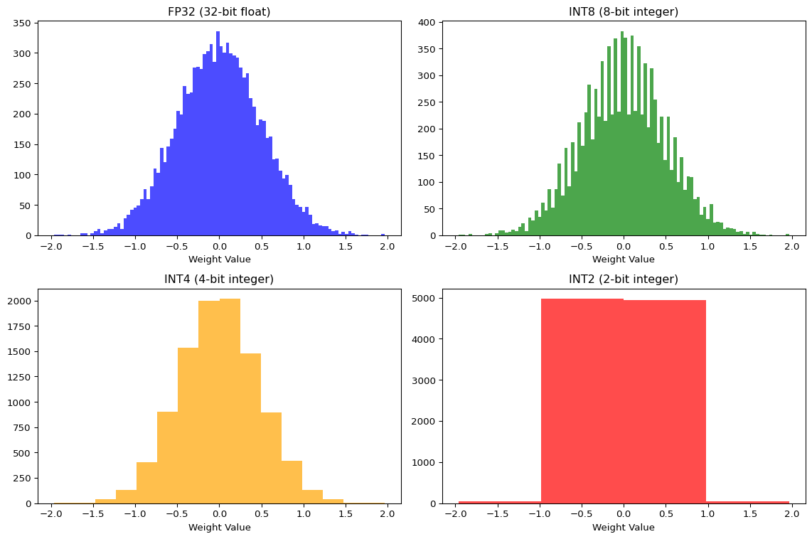
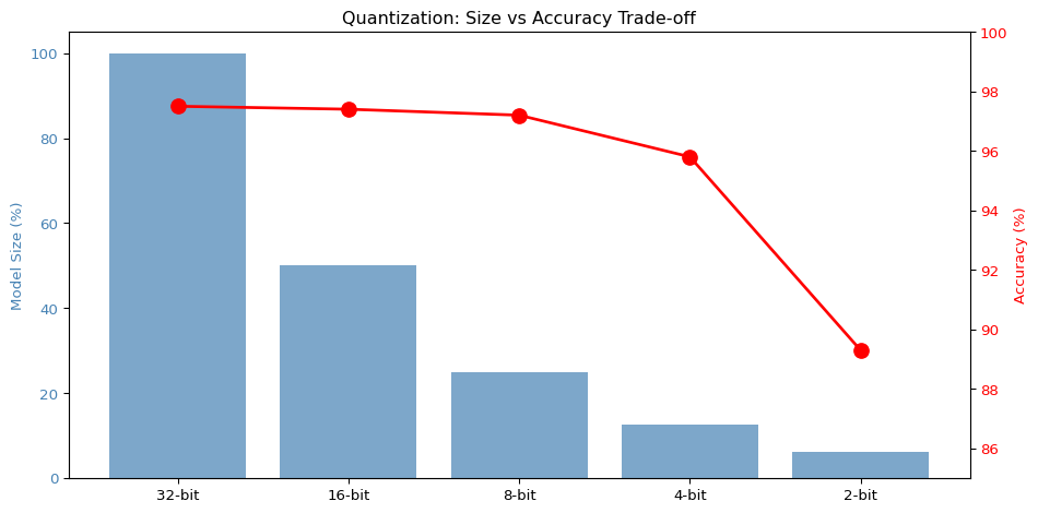
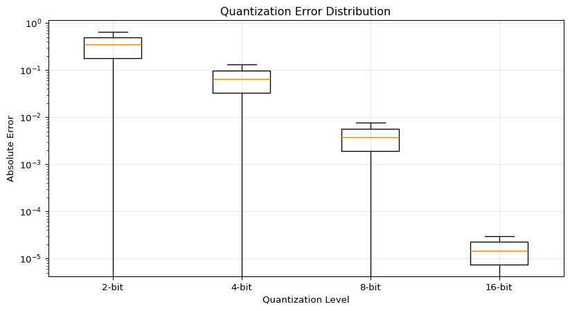
--- title: "Quantization Explorer" subtitle: "LAB03: TensorFlow Lite and Quantization" --- ## Interactive Quantization Visualization ## Concept from LAB03 [ PDF book ](../downloads/Edge-Analytics-Lab-Book-v1.0.0.pdf) .## Interactive Quantization Simulator ```{ojs} //| echo: false // Input controls viewof bitWidth = Inputs.range([2, 32], { value: 8, step: 1, label: "Bit Width", description: "Number of bits for quantized values" }) viewof modelSizeMB = Inputs.range([1, 100], { value: 10, step: 1, label: "Base Model Size (MB)", description: "Original FP32 model size" }) viewof numWeights = Inputs.range([1000, 1000000], { value: 100000, step: 1000, label: "Number of Weights", description: "Total parameters in the model" }) ``` ```{ojs} //| echo: false // Calculate quantization metrics quantizedSizeMB = (modelSizeMB * bitWidth) / 32 // Estimated accuracy based on typical results baseAccuracy = 97.5 accuracyLoss = bitWidth >= 16 ? 0.1 : bitWidth >= 8 ? 0.3 : bitWidth >= 4 ? 1.7 : 8.2 quantizedAccuracy = baseAccuracy - accuracyLoss sizeReduction = ((1 - quantizedSizeMB / modelSizeMB) * 100) memoryBytes = (numWeights * bitWidth) / 8 // Quantization error simulation quantizationError = 1 / Math.pow(2, bitWidth) html`<div style="background: linear-gradient(135deg, #667eea 0%, #764ba2 100%); padding: 25px; border-radius: 10px; color: white; margin: 20px 0;"> <h3 style="margin-top: 0;">Quantization Results: ${bitWidth}-bit</h3> <div style="display: grid; grid-template-columns: repeat(auto-fit, minmax(180px, 1fr)); gap: 20px; margin-top: 15px;"> <div style="background: rgba(255,255,255,0.1); padding: 15px; border-radius: 8px;"> <div style="font-size: 1.8em; font-weight: bold;">${quantizedSizeMB.toFixed(2)} MB</div> <div style="opacity: 0.9;">Model Size</div> <div style="font-size: 0.9em; margin-top: 5px; opacity: 0.8;">↓ ${sizeReduction.toFixed(1)}% reduction</div> </div> <div style="background: rgba(255,255,255,0.1); padding: 15px; border-radius: 8px;"> <div style="font-size: 1.8em; font-weight: bold;">${quantizedAccuracy.toFixed(2)}%</div> <div style="opacity: 0.9;">Accuracy</div> <div style="font-size: 0.9em; margin-top: 5px; opacity: 0.8;">↓ ${accuracyLoss.toFixed(2)}% loss</div> </div> <div style="background: rgba(255,255,255,0.1); padding: 15px; border-radius: 8px;"> <div style="font-size: 1.8em; font-weight: bold;">${(memoryBytes / 1024).toFixed(0)} KB</div> <div style="opacity: 0.9;">Memory Usage</div> <div style="font-size: 0.9em; margin-top: 5px; opacity: 0.8;">${numWeights.toLocaleString()} weights</div> </div> <div style="background: rgba(255,255,255,0.1); padding: 15px; border-radius: 8px;"> <div style="font-size: 1.8em; font-weight: bold;">${quantizationError.toExponential(2)}</div> <div style="opacity: 0.9;">Quant. Error</div> <div style="font-size: 0.9em; margin-top: 5px; opacity: 0.8;">Per value</div> </div> </div> </div>` ``` ## Bit Width Comparison ```{ojs} //| echo: false bitWidthOptions = [2, 4, 8, 16, 32] comparisonData = bitWidthOptions.map(bits => { const sizeMB = (modelSizeMB * bits) / 32 const accLoss = bits >= 16 ? 0.1 : bits >= 8 ? 0.3 : bits >= 4 ? 1.7 : 8.2 const acc = baseAccuracy - accLoss return { bits: `${bits}-bit`, bitsNum: bits, size: sizeMB, accuracy: acc, sizePercent: (sizeMB / modelSizeMB) * 100, isCurrent: bits === bitWidth } }) Plot.plot({ height: 400, marginLeft: 60, marginBottom: 60, x: {label: "Bit Width"}, y: {label: "Model Size (MB)", grid: true}, color: {domain: [false, true], range: ["#94a3b8", "#ef4444"]}, marks: [ Plot.barY(comparisonData, { x: "bits", y: "size", fill: "isCurrent", title: d => `${d.bits}: ${d.size.toFixed(2)} MB (${d.sizePercent.toFixed(0)}% of FP32)` }), Plot.text(comparisonData, { x: "bits", y: "size", text: d => `${d.size.toFixed(1)} MB`, dy: -10, fontSize: 11 }), Plot.ruleY([0]) ] }) ``` ## Accuracy vs Model Size Trade-off ```{ojs} //| echo: false Plot.plot({ height: 400, marginLeft: 60, marginRight: 60, x: {label: "Model Size (MB)"}, y: {label: "Accuracy (%)", domain: [85, 100]}, color: {domain: [false, true], range: ["#0ea5e9", "#ef4444"]}, marks: [ Plot.line(comparisonData, { x: "size", y: "accuracy", stroke: "#0ea5e9", strokeWidth: 3, curve: "natural" }), Plot.dot(comparisonData, { x: "size", y: "accuracy", fill: "isCurrent", r: d => d.isCurrent ? 10 : 6, title: d => `${d.bits}: ${d.accuracy.toFixed(2)}% accuracy, ${d.size.toFixed(2)} MB` }), Plot.text(comparisonData, { x: "size", y: "accuracy", text: "bits", dy: -15, fontSize: 10 }), Plot.gridY({stroke: "#e5e7eb", strokeOpacity: 0.5}), Plot.ruleY([90, 95], {stroke: "#94a3b8", strokeDasharray: "4,4"}) ] }) ``` ## Quantization Levels Visualization ```{ojs} //| echo: false // Generate sample weight distribution numSamples = 200 weightRange = 3 sampleWeights = Array.from({length: numSamples}, () => (Math.random() - 0.5) * 2 * weightRange ) // Quantize weights function quantizeValue(value, bits, minVal, maxVal) { const levels = Math.pow(2, bits) const scale = (maxVal - minVal) / (levels - 1) const quantized = Math.round((value - minVal) / scale) * scale + minVal return Math.max(minVal, Math.min(maxVal, quantized)) } minWeight = -weightRange maxWeight = weightRange quantizedWeights = sampleWeights.map(w => quantizeValue(w, bitWidth, minWeight, maxWeight) ) // Create histogram data histogramData = { const data = [] for (let i = 0; i < numSamples; i++) { data.push({ type: "Original (FP32)", value: sampleWeights[i] }) data.push({ type: `Quantized (${bitWidth}-bit)`, value: quantizedWeights[i] }) } return data } Plot.plot({ height: 350, x: {label: "Weight Value", domain: [-weightRange, weightRange]}, y: {label: "Count"}, color: {domain: ["Original (FP32)", `Quantized (${bitWidth}-bit)`], range: ["#3b82f6", "#f59e0b"]}, marks: [ Plot.rectY( histogramData, Plot.binX( {y: "count"}, { x: "value", fill: "type", thresholds: 40, mixBlendMode: "multiply" } ) ), Plot.ruleY([0]) ], facet: { data: histogramData, y: "type", marginLeft: 150 } }) ``` ## Quantization Error Distribution ```{ojs} //| echo: false errorData = sampleWeights.map((original, i) => ({ index: i, original: original, quantized: quantizedWeights[i], error: Math.abs(original - quantizedWeights[i]) })) Plot.plot({ height: 300, x: {label: "Sample Index"}, y: {label: "Absolute Error", type: "log"}, marks: [ Plot.dot(errorData, { x: "index", y: d => d.error + 1e-6, fill: "#ef4444", r: 2, opacity: 0.6 }), Plot.ruleY([quantizationError], { stroke: "#0ea5e9", strokeWidth: 2, strokeDasharray: "4,4" }), Plot.text([{x: numSamples * 0.95, y: quantizationError, label: "Expected Error"}], { x: "x", y: "y", text: "label", textAnchor: "end", dy: -8, fill: "#0ea5e9", fontSize: 11 }) ] }) ``` ## Weight Distribution Comparison ```{python} #| label: fig-quantization #| fig-cap: "Effect of quantization on weight distribution" import numpy as npimport matplotlib.pyplot as plt# Simulate FP32 weights (normal distribution) 42 )= np.random.randn(10000 ) * 0.5 # Quantize to different bit widths def quantize(weights, bits):= weights.min (), weights.max ()= (max_val - min_val) / (2 ** bits - 1 )= np.round ((weights - min_val) / scale) * scale + min_valreturn quantized= plt.subplots(2 , 2 , figsize= (12 , 8 ))# FP32 0 , 0 ].hist(fp32_weights, bins= 100 , alpha= 0.7 , color= 'blue' )0 , 0 ].set_title('FP32 (32-bit float)' )0 , 0 ].set_xlabel('Weight Value' )# INT8 = quantize(fp32_weights, 8 )0 , 1 ].hist(int8_weights, bins= 100 , alpha= 0.7 , color= 'green' )0 , 1 ].set_title('INT8 (8-bit integer)' )0 , 1 ].set_xlabel('Weight Value' )# INT4 = quantize(fp32_weights, 4 )1 , 0 ].hist(int4_weights, bins= 16 , alpha= 0.7 , color= 'orange' )1 , 0 ].set_title('INT4 (4-bit integer)' )1 , 0 ].set_xlabel('Weight Value' )# INT2 = quantize(fp32_weights, 2 )1 , 1 ].hist(int2_weights, bins= 4 , alpha= 0.7 , color= 'red' )1 , 1 ].set_title('INT2 (2-bit integer)' )1 , 1 ].set_xlabel('Weight Value' )``` ## Size vs Accuracy Trade-off ```{python} #| label: fig-tradeoff #| fig-cap: "Model size vs accuracy for different quantization levels" # Simulated data based on typical results = [32 , 16 , 8 , 4 , 2 ]= [100 , 50 , 25 , 12.5 , 6.25 ] # Relative size (%) = [97.5 , 97.4 , 97.2 , 95.8 , 89.3 ] # Typical MNIST accuracy = plt.subplots(figsize= (10 , 5 ))# Model size bars = ax1.bar(range (len (bit_widths)), model_sizes, color= 'steelblue' , alpha= 0.7 )range (len (bit_widths)))f' { b} -bit' for b in bit_widths])'Model Size (%)' , color= 'steelblue' )= 'y' , labelcolor= 'steelblue' )# Accuracy line = ax1.twinx()range (len (bit_widths)), accuracies, 'ro-' , linewidth= 2 , markersize= 10 )'Accuracy (%)' , color= 'red' )= 'y' , labelcolor= 'red' )85 , 100 )'Quantization: Size vs Accuracy Trade-off' )``` ## Quantization Error Analysis ```{python} #| label: fig-error #| fig-cap: "Quantization error by bit width" = []for bits in [2 , 4 , 8 , 16 ]:= quantize(fp32_weights, bits)= np.abs (fp32_weights - quantized)= plt.subplots(figsize= (10 , 5 ))= ax.boxplot(errors, labels= ['2-bit' , '4-bit' , '8-bit' , '16-bit' ])'Absolute Error' )'Quantization Level' )'Quantization Error Distribution' )'log' )True , alpha= 0.3 )``` ## Key Insights ## Recommendation - 4x size reduction- Minimal accuracy loss- Hardware acceleration on most devices## Try It Yourself 1. Open the [ LAB03 notebook ](https://github.com/ngcharithperera/edge-analytics-lab-book/blob/main/notebooks/LAB03_tflite_quantization.ipynb) 2. Train a model on CIFAR-103. Apply different quantization methods4. Compare file sizes and accuracy## Related Sections in PDF Book - Section 3.1: Why Quantization?- Section 3.2: Quantization Types- Section 3.3: Post-Training Quantization- Section 3.4: Quantization-Aware Training