For detailed theoretical foundations, mathematical proofs, and algorithm derivations, see Chapter 2: Neural Network Training Fundamentals in the PDF textbook.
The PDF chapter includes: - Complete mathematical derivations of backpropagation - Detailed loss function formulations and proofs - In-depth coverage of gradient descent variants - Comprehensive CNN architecture theory - Extended theoretical examples and convergence analysis
Define and compute common loss functions for regression and classification
Implement gradient descent and understand how learning rate affects convergence
Build and train simple neural networks and CNNs in TensorFlow/Keras
Interpret training/validation curves and diagnose under/overfitting
Theory Summary
How Neural Networks Learn
Neural networks learn through an iterative optimization process that adjusts millions of parameters to minimize prediction errors. Understanding this process is essential for diagnosing training problems and building effective edge ML models.
Loss Functions - Measuring Mistakes: A loss function quantifies how wrong your model’s predictions are. For regression tasks (predicting numbers), we use Mean Squared Error (MSE) which penalizes large errors more heavily. For classification (predicting categories), we use Cross-Entropy Loss which measures the difference between predicted probabilities and true labels. Lower loss always means better predictions.
Gradient Descent - The Optimization Engine: Gradient descent is an algorithm that automatically finds parameter values that minimize loss. It works by computing the gradient (derivative) of the loss with respect to each parameter, then taking small steps in the opposite direction. The learning rate controls step size - too large causes oscillation, too small causes slow convergence. Think of it like walking downhill in fog: you can’t see the bottom, but you can feel the slope and take steps downward.
Neural Network Architecture: A neural network stacks multiple layers of simple operations (\(y = wx + b\)) with non-linear activation functions between them. Each layer learns increasingly abstract features: early layers detect edges and textures, middle layers combine them into shapes, and final layers recognize complete objects. This hierarchical feature learning is what makes neural networks powerful.
Key Concepts at a Glance
Core Concepts
Loss Function: Single number measuring prediction error (lower = better)
Gradient: Derivative showing direction to adjust parameters for improvement
Overfitting: Model memorizes training data but fails on new data
Regularization: Techniques (dropout, L2 penalty) to prevent overfitting
Common Pitfalls
Mistakes to Avoid
Forgetting to Normalize Inputs: The most common training failure is feeding unnormalized data to neural networks. If pixel values are 0-255 instead of 0-1, gradients become 255× larger, causing training instability or divergence. Always normalize: x = x / 255.0 for images.
Using Wrong Loss for Task Type: Mean Squared Error (MSE) is for regression (predicting continuous values). Cross-Entropy is for classification (predicting categories). Using MSE for classification or cross-entropy for regression will cause training to fail silently with poor results.
Learning Rate Too High or Too Low: Learning rate = 1.0 typically causes wild oscillation and divergence. Learning rate = 0.00001 makes training painfully slow (thousands of epochs). Start with 0.001 or 0.01 and adjust based on loss curves.
Not Splitting Train/Validation Data: Training and evaluating on the same data gives misleadingly high accuracy. Always hold out 10-20% of data for validation to detect overfitting. Use validation_split=0.2 in Keras or manually split your dataset.
Ignoring Training Curves: If validation loss increases while training loss decreases, you’re overfitting. If both losses are high, your model is underfitting. Always plot loss curves to diagnose issues early.
Quick Reference
Key Formulas
Mean Squared Error (Regression):\[\text{MSE} = \frac{1}{n}\sum_{i=1}^{n}(y_i - \hat{y}_i)^2\]
Cross-Entropy Loss (Classification):\[\text{Loss} = -\frac{1}{n}\sum_{i=1}^{n}\sum_{c=1}^{C} y_{ic} \log(\hat{y}_{ic})\]
Gradient Descent Update Rule:\[w_{new} = w_{old} - \alpha \cdot \frac{\partial L}{\partial w}\] where \(\alpha\) is the learning rate
Parameter Count for Dense Layer:\[\text{params} = (\text{input\_size} + 1) \times \text{output\_size}\] The “+1” accounts for bias terms
Memory for Float32 Model:\[\text{Memory (bytes)} = \text{parameters} \times 4\]
Important Parameter Values
Hyperparameter
Typical Range
Notes
Learning Rate
0.001 - 0.1
Start with 0.01, adjust by 10×
Batch Size
16 - 128
Smaller = noisier gradients but less memory
Epochs
5 - 100
Stop when validation loss stops improving
Hidden Layer Size
16 - 512
Larger = more capacity but slower
Dropout Rate
0.2 - 0.5
Prevents overfitting (0.5 = drop 50% neurons)
Common Activation Functions: - ReLU: max(0, x) - Default choice, fast, works well - Sigmoid: 1/(1+e^-x) - Output 0-1, used for binary classification - Softmax: Normalizes to probabilities - used for multi-class output - Tanh: tanh(x) - Output -1 to 1, centered around zero
Links to PDF Sections
For deeper understanding, see these sections in Chapter 2 PDF:
Section 2.1: Exploring Loss Functions (pages 21-24)
Run these interactive examples directly in your browser to build intuition before diving into the full notebook.
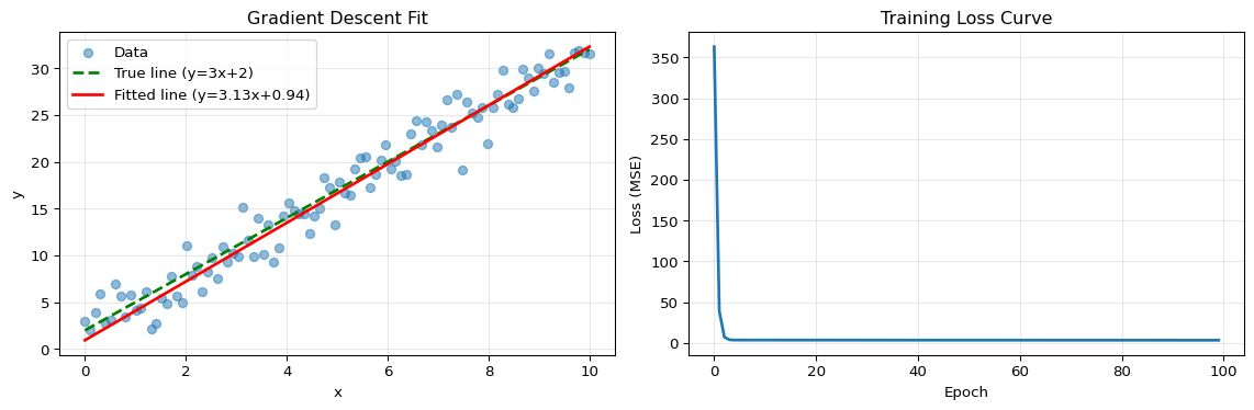
Example 1: Gradient Descent from Scratch
Code
import numpy as npimport matplotlib.pyplot as plt# Generate synthetic data: y = 3x + 2 + noisenp.random.seed(42)X = np.linspace(0, 10, 100)y_true =3* X +2y = y_true + np.random.randn(100) *2# Initialize parametersw =0.0# weightb =0.0# biaslearning_rate =0.01epochs =100# Track loss historyloss_history = []# Gradient descentfor epoch inrange(epochs):# Forward pass: predictions y_pred = w * X + b# Compute loss (MSE) loss = np.mean((y - y_pred) **2) loss_history.append(loss)# Compute gradients grad_w =-2* np.mean((y - y_pred) * X) grad_b =-2* np.mean(y - y_pred)# Update parameters w = w - learning_rate * grad_w b = b - learning_rate * grad_b# Visualize resultsfig, (ax1, ax2) = plt.subplots(1, 2, figsize=(12, 4))# Plot 1: Data and fitted lineax1.scatter(X, y, alpha=0.5, label='Data')ax1.plot(X, y_true, 'g--', label='True line (y=3x+2)', linewidth=2)ax1.plot(X, w * X + b, 'r-', label=f'Fitted line (y={w:.2f}x+{b:.2f})', linewidth=2)ax1.set_xlabel('x')ax1.set_ylabel('y')ax1.set_title('Gradient Descent Fit')ax1.legend()ax1.grid(True, alpha=0.3)# Plot 2: Loss over epochsax2.plot(loss_history, linewidth=2)ax2.set_xlabel('Epoch')ax2.set_ylabel('Loss (MSE)')ax2.set_title('Training Loss Curve')ax2.grid(True, alpha=0.3)plt.tight_layout()plt.show()print(f"Final parameters: w={w:.4f}, b={b:.4f}")print(f"True parameters: w=3.0000, b=2.0000")print(f"Final loss: {loss_history[-1]:.4f}")print(f"\nKey insight: Gradient descent found parameters close to the true values!")
Final parameters: w=3.1348, b=0.9415
True parameters:  w=3.0000, b=2.0000
Final loss: 3.3899

Key insight: Gradient descent found parameters close to the true values!
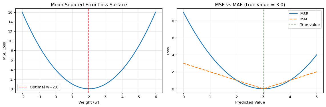
Example 2: Loss Function Visualization
Code
import numpy as npimport matplotlib.pyplot as plt# Generate classification and regression examplesnp.random.seed(42)# Regression exampley_true_reg = np.array([1.0, 2.0, 3.0, 4.0, 5.0])y_pred_reg = np.array([1.2, 2.1, 2.8, 4.3, 4.9])# Classification example (3 classes)y_true_class = np.array([[1, 0, 0], [0, 1, 0], [0, 0, 1], [1, 0, 0], [0, 1, 0]])y_pred_class = np.array([[0.8, 0.1, 0.1], [0.2, 0.7, 0.1], [0.1, 0.2, 0.7], [0.6, 0.3, 0.1], [0.1, 0.8, 0.1]])# Compute lossesmse = np.mean((y_true_reg - y_pred_reg) **2)mae = np.mean(np.abs(y_true_reg - y_pred_reg))# Cross-entropy loss (clip to avoid log(0))y_pred_clipped = np.clip(y_pred_class, 1e-7, 1-1e-7)cross_entropy =-np.mean(np.sum(y_true_class * np.log(y_pred_clipped), axis=1))# Visualize loss surfaces for simple casefig, (ax1, ax2) = plt.subplots(1, 2, figsize=(12, 4))# MSE loss surface for y = wx (simple linear)w_range = np.linspace(-2, 6, 100)mse_surface = [(np.mean(([2.0] - w * np.array([1.0])) **2)) for w in w_range]ax1.plot(w_range, mse_surface, linewidth=2)ax1.axvline(x=2.0, color='r', linestyle='--', label='Optimal w=2.0')ax1.set_xlabel('Weight (w)')ax1.set_ylabel('MSE Loss')ax1.set_title('Mean Squared Error Loss Surface')ax1.legend()ax1.grid(True, alpha=0.3)# Compare different loss magnitudespredictions = np.linspace(0, 5, 100)true_value =3.0mse_curve = (predictions - true_value) **2mae_curve = np.abs(predictions - true_value)ax2.plot(predictions, mse_curve, label='MSE', linewidth=2)ax2.plot(predictions, mae_curve, label='MAE', linewidth=2, linestyle='--')ax2.axvline(x=true_value, color='g', linestyle=':', alpha=0.5, label='True value')ax2.set_xlabel('Predicted Value')ax2.set_ylabel('Loss')ax2.set_title('MSE vs MAE (true value = 3.0)')ax2.legend()ax2.grid(True, alpha=0.3)plt.tight_layout()plt.show()print("LOSS FUNCTION COMPARISON")print("="*50)print(f"\nRegression Losses:")print(f" MSE (Mean Squared Error): {mse:.4f}")print(f" MAE (Mean Absolute Error): {mae:.4f}")print(f"\nClassification Loss:")print(f" Cross-Entropy Loss: {cross_entropy:.4f}")print(f"\nKey insight: MSE penalizes large errors more heavily (squared term)!")
LOSS FUNCTION COMPARISON
==================================================

Regression Losses:
  MSE (Mean Squared Error):     0.0380
  MAE (Mean Absolute Error):    0.1800

Classification Loss:
  Cross-Entropy Loss:           0.3341

Key insight: MSE penalizes large errors more heavily (squared term)!
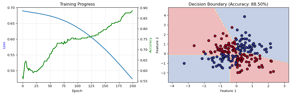
Final loss: 0.4738
Final accuracy: 88.50%

Key insight: Neural networks learn nonlinear decision boundaries!
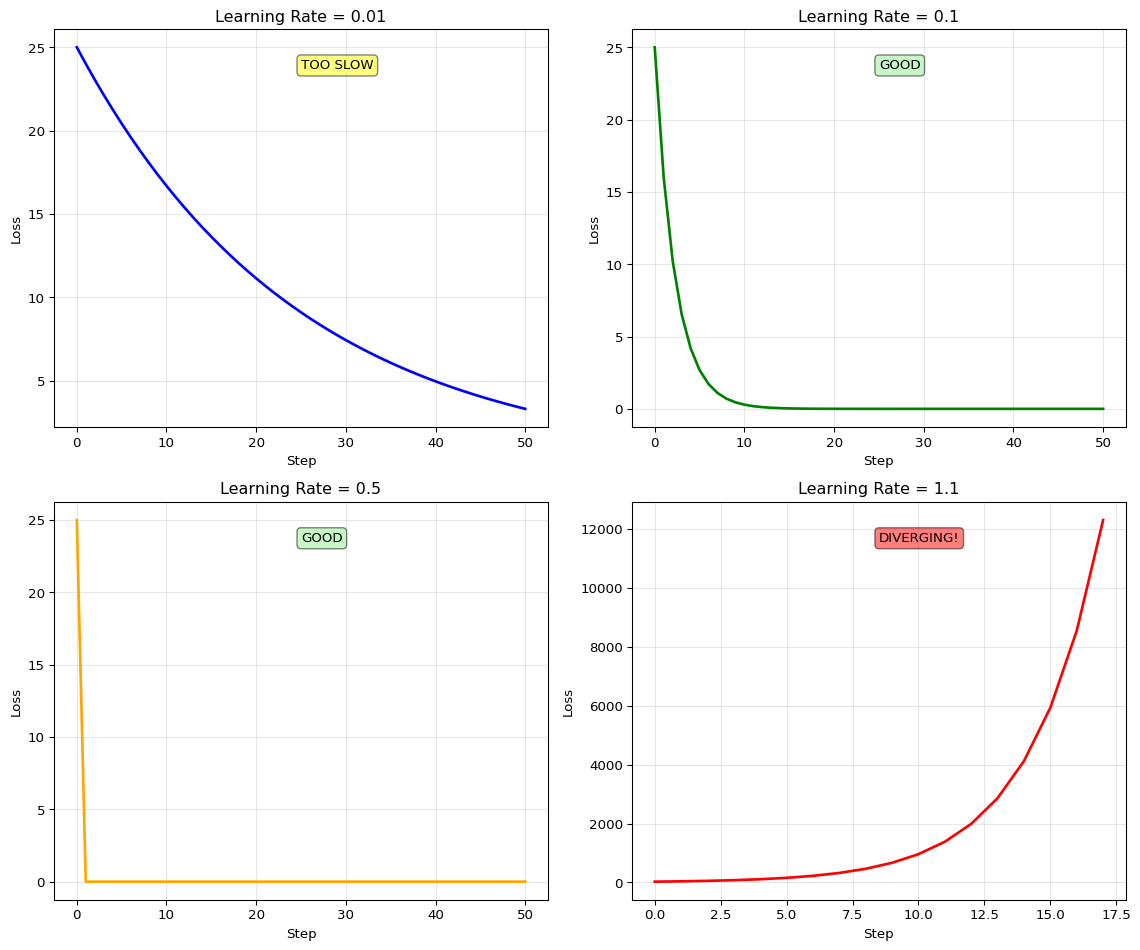
Example 4: Learning Rate Comparison
Code
import numpy as npimport matplotlib.pyplot as plt# Simple quadratic loss surface: L(w) = (w - 5)^2def loss_fn(w):return (w -5) **2def gradient_fn(w):return2* (w -5)# Test different learning rateslearning_rates = [0.01, 0.1, 0.5, 1.1]colors = ['blue', 'green', 'orange', 'red']n_steps =50fig, axes = plt.subplots(2, 2, figsize=(12, 10))axes = axes.flatten()for idx, (lr, color) inenumerate(zip(learning_rates, colors)): w =0.0# Start far from optimum w_history = [w] loss_history = [loss_fn(w)]for step inrange(n_steps): grad = gradient_fn(w) w = w - lr * grad w_history.append(w) loss_history.append(loss_fn(w))# Stop if divergingifabs(w) >100:break# Plot loss trajectory ax = axes[idx] ax.plot(loss_history, linewidth=2, color=color) ax.set_xlabel('Step') ax.set_ylabel('Loss') ax.set_title(f'Learning Rate = {lr}') ax.grid(True, alpha=0.3)# Add status textif lr <0.1: status ="TOO SLOW" ax.text(0.5, 0.9, status, transform=ax.transAxes, bbox=dict(boxstyle='round', facecolor='yellow', alpha=0.5))elif lr >1.0: status ="DIVERGING!" ax.text(0.5, 0.9, status, transform=ax.transAxes, bbox=dict(boxstyle='round', facecolor='red', alpha=0.5))else: status ="GOOD" ax.text(0.5, 0.9, status, transform=ax.transAxes, bbox=dict(boxstyle='round', facecolor='lightgreen', alpha=0.5))plt.tight_layout()plt.show()print("LEARNING RATE COMPARISON")print("="*60)for lr in learning_rates: w =0.0for step inrange(50): w = w - lr * gradient_fn(w)ifabs(w) >100:print(f"LR={lr:4.2f}: DIVERGED at step {step}")breakelse: final_loss = loss_fn(w)print(f"LR={lr:4.2f}: Converged to w={w:.4f}, loss={final_loss:.4f}")print("\nKey insights:")print(" • LR=0.01: Too slow, needs many iterations")print(" • LR=0.1: Good balance, stable convergence")print(" • LR=0.5: Fast but may oscillate")print(" • LR=1.1: Too large, diverges!")
LEARNING RATE COMPARISON
============================================================
LR=0.01: Converged to w=3.1792, loss=3.3155
LR=0.10: Converged to w=4.9999, loss=0.0000
LR=0.50: Converged to w=5.0000, loss=0.0000
LR=1.10: DIVERGED at step 16

Key insights:
  • LR=0.01: Too slow, needs many iterations
  • LR=0.1:  Good balance, stable convergence
  • LR=0.5:  Fast but may oscillate
  • LR=1.1:  Too large, diverges!
Interactive Notebook
The notebook below contains runnable code for all Level 1 activities.
LAB02: Machine Learning Foundations for Edge
Learning Objectives: - Understand neural network architecture fundamentals - Train simple models on synthetic datasets - Explore loss functions and gradient descent - Export models to TensorFlow Lite format
Three-Tier Approach: - Level 1 (This Notebook): Train and visualize models on laptop - Level 2 (Simulator): Use TensorFlow Playground for visualization - Level 3 (Device): Deploy quantized model to microcontroller
1. Setup
2. Understanding Neural Networks
A neural network consists of: - Input layer: Receives raw data features - Hidden layers: Transform features through weighted connections - Output layer: Produces predictions
Each connection has a weight that is learned during training.
3. Create a Toy Dataset
We’ll use a simple 2D classification problem that’s easy to visualize.
4. Build a Simple Neural Network
We’ll create a tiny network suitable for edge deployment: - 2 input features - 1 hidden layer with 8 neurons - 2 output classes
5. Understanding Loss Functions
The loss function measures how wrong our predictions are: - Cross-entropy loss: For classification problems - Mean squared error: For regression problems
Goal: Minimize the loss by adjusting weights.
6. Training: Gradient Descent in Action
Training process: 1. Forward pass: Compute predictions 2. Compute loss 3. Backward pass: Compute gradients 4. Update weights 5. Repeat
7. Visualize Decision Boundary
8. Export to TensorFlow Lite
For edge deployment, we convert to TFLite format which is: - Smaller (optimized for mobile/embedded) - Faster (quantized operations) - Compatible with microcontrollers
9. Test TFLite Model
10. Checkpoint Questions
Why does the loss decrease during training?
What happens if you increase the number of hidden neurons from 8 to 32?
How does training time change?
How does accuracy change?
How does model size change?
What’s the purpose of the validation set?
Why is the INT8 model smaller than the float32 model?
Test your understanding before proceeding to the exercises.
Question 1: Why would you use Cross-Entropy loss instead of MSE for a 10-class image classification problem?
Answer: Cross-Entropy loss is designed for classification tasks and measures the difference between predicted probability distributions and true labels. MSE treats class labels as numeric values (0, 1, 2…) which doesn’t make sense - the “distance” between class 0 and class 2 has no meaning. Cross-Entropy properly handles probability outputs from softmax and provides better gradients for classification. Using MSE for classification leads to poor convergence and lower accuracy.
Question 2: Calculate the number of parameters in a Dense layer with 128 inputs and 64 outputs.
Answer: Parameters = (input_size + 1) × output_size = (128 + 1) × 64 = 129 × 64 = 8,256 parameters. The “+1” accounts for bias terms (one bias per output neuron). In float32, this layer requires 8,256 × 4 = 33,024 bytes (32.25 KB). After int8 quantization, it reduces to 8,256 bytes (8.06 KB).
Question 3: Your model’s training loss decreases steadily but validation loss starts increasing after epoch 10. What’s happening and what should you do?
Answer: This is overfitting - the model is memorizing training data instead of learning generalizable patterns. After epoch 10, it performs worse on unseen validation data. Solutions: (1) Stop training at epoch 10 (early stopping), (2) Add regularization (L2 penalty, dropout), (3) Increase training data size, (4) Reduce model complexity (fewer layers/neurons), or (5) Add data augmentation. Always monitor validation loss and stop when it stops improving.
Question 4: You set learning_rate=1.0 and the loss oscillates wildly between 0.1 and 100. What’s wrong?
Answer: The learning rate is too high. Large steps cause gradient descent to overshoot the minimum and bounce around the loss surface wildly. The loss may even diverge to infinity. Solution: Reduce learning rate by 10× or 100×. Start with 0.01 or 0.001 and adjust based on loss curves. If loss decreases smoothly, the rate is good. If it plateaus quickly, try increasing slightly. A good learning rate shows steady decrease without oscillation.
Question 5: Why must you normalize image inputs (pixel_values / 255.0) before training?
Answer: Neural networks expect inputs in a consistent, small range (typically 0-1 or -1 to 1). Raw pixel values (0-255) cause several problems: (1) Gradients become 255× larger, leading to training instability and divergence, (2) Initial random weights (typically -0.1 to 0.1) are completely wrong for 0-255 scale, (3) Optimization is much slower because the loss surface is poorly conditioned. Normalization ensures all input features have similar scales, enabling stable and efficient training.
There is no dedicated on-device deployment in LAB02. Instead:
LAB03 introduces TFLite conversion and quantization for edge deployment
LAB05 shows how to take a trained model and deploy it to Arduino/MCUs
If you want an early challenge, you can:
Train a small MNIST model in this lab’s notebook
Follow LAB03 to convert and quantize it to .tflite
Follow LAB05 to integrate that .tflite model into an MCU project
Visual Troubleshooting
Training Loss Not Decreasing
flowchart TD
    A[Loss not decreasing] --> B{Loss value?}
    B -->|NaN| C[Gradient explosion:<br/>Reduce learning rate 10x<br/>Add gradient clipping<br/>Check for NaN in data]
    B -->|Constant high| D{Learning rate?}
    D -->|Too small| E[Increase LR:<br/>Try 1e-3 for Adam<br/>Try 0.01 for SGD]
    D -->|Reasonable| F{Data normalized?}
    F -->|No| G[Normalize inputs:<br/>x = x / 255.0 images<br/>StandardScaler tabular<br/>Mean 0 std 1]
    F -->|Yes| H{Check labels}
    H -->|Wrong format| I[Fix labels:<br/>One-hot encode<br/>Balance classes<br/>Verify ground truth]

    style A fill:#ff6b6b
    style C fill:#4ecdc4
    style E fill:#4ecdc4
    style G fill:#4ecdc4
    style I fill:#4ecdc4
Overfitting Problems
flowchart TD
    A[Train acc high<br/>Val acc low] --> B{Gap size?}
    B -->|>20%| C[Severe overfitting]
    B -->|10-20%| D[Moderate]
    C --> E{Dataset size?}
    E -->|<100/class| F[Collect more data:<br/>Aim 500+ per class<br/>Critical for deep learning]
    E -->|Adequate| G{Using augmentation?}
    G -->|No| H[Add augmentation:<br/>Flips rotations<br/>Noise injection<br/>Time warping]
    G -->|Yes| I[Add regularization:<br/>L2 weight decay 1e-4<br/>Dropout 0.3-0.5<br/>Early stopping]
    D --> G

    style A fill:#ff6b6b
    style F fill:#4ecdc4
    style H fill:#4ecdc4
    style I fill:#4ecdc4
---title: "LAB02: Machine Learning Foundations"subtitle: "Neural Networks and Training Basics"---::: {.callout-note}## PDF Textbook ReferenceFor detailed theoretical foundations, mathematical proofs, and algorithm derivations, see **Chapter 2: Neural Network Training Fundamentals** in the [PDF textbook](../downloads/Edge-Analytics-Lab-Book-v1.0.0.pdf).The PDF chapter includes:- Complete mathematical derivations of backpropagation- Detailed loss function formulations and proofs- In-depth coverage of gradient descent variants- Comprehensive CNN architecture theory- Extended theoretical examples and convergence analysis:::[](https://colab.research.google.com/github/ngcharithperera/edge-analytics-lab-book/blob/main/notebooks/LAB02_ml_foundations.ipynb)[Download Notebook](https://raw.githubusercontent.com/ngcharithperera/edge-analytics-lab-book/main/notebooks/LAB02_ml_foundations.ipynb)## Learning ObjectivesBy the end of this lab you will be able to:- Define and compute common loss functions for regression and classification- Implement gradient descent and understand how learning rate affects convergence- Build and train simple neural networks and CNNs in TensorFlow/Keras- Interpret training/validation curves and diagnose under/overfitting## Theory Summary### How Neural Networks LearnNeural networks learn through an iterative optimization process that adjusts millions of parameters to minimize prediction errors. Understanding this process is essential for diagnosing training problems and building effective edge ML models.**Loss Functions - Measuring Mistakes:** A loss function quantifies how wrong your model's predictions are. For regression tasks (predicting numbers), we use Mean Squared Error (MSE) which penalizes large errors more heavily. For classification (predicting categories), we use Cross-Entropy Loss which measures the difference between predicted probabilities and true labels. Lower loss always means better predictions.**Gradient Descent - The Optimization Engine:** Gradient descent is an algorithm that automatically finds parameter values that minimize loss. It works by computing the gradient (derivative) of the loss with respect to each parameter, then taking small steps in the opposite direction. The learning rate controls step size - too large causes oscillation, too small causes slow convergence. Think of it like walking downhill in fog: you can't see the bottom, but you can feel the slope and take steps downward.**Neural Network Architecture:** A neural network stacks multiple layers of simple operations ($y = wx + b$) with non-linear activation functions between them. Each layer learns increasingly abstract features: early layers detect edges and textures, middle layers combine them into shapes, and final layers recognize complete objects. This hierarchical feature learning is what makes neural networks powerful.## Key Concepts at a Glance::: {.callout-note icon=false}## Core Concepts- **Loss Function**: Single number measuring prediction error (lower = better)- **Gradient**: Derivative showing direction to adjust parameters for improvement- **Learning Rate**: Step size for gradient descent updates (typically 0.001 - 0.1)- **Epoch**: One complete pass through the entire training dataset- **Activation Functions**: Non-linearities (ReLU, sigmoid, softmax) enabling complex patterns- **Overfitting**: Model memorizes training data but fails on new data- **Regularization**: Techniques (dropout, L2 penalty) to prevent overfitting:::## Common Pitfalls::: {.callout-warning}## Mistakes to Avoid**Forgetting to Normalize Inputs**: The most common training failure is feeding unnormalized data to neural networks. If pixel values are 0-255 instead of 0-1, gradients become 255× larger, causing training instability or divergence. Always normalize: `x = x / 255.0` for images.**Using Wrong Loss for Task Type**: Mean Squared Error (MSE) is for regression (predicting continuous values). Cross-Entropy is for classification (predicting categories). Using MSE for classification or cross-entropy for regression will cause training to fail silently with poor results.**Learning Rate Too High or Too Low**: Learning rate = 1.0 typically causes wild oscillation and divergence. Learning rate = 0.00001 makes training painfully slow (thousands of epochs). Start with 0.001 or 0.01 and adjust based on loss curves.**Not Splitting Train/Validation Data**: Training and evaluating on the same data gives misleadingly high accuracy. Always hold out 10-20% of data for validation to detect overfitting. Use `validation_split=0.2` in Keras or manually split your dataset.**Ignoring Training Curves**: If validation loss increases while training loss decreases, you're overfitting. If both losses are high, your model is underfitting. Always plot loss curves to diagnose issues early.:::## Quick Reference### Key Formulas**Mean Squared Error (Regression):**$$\text{MSE} = \frac{1}{n}\sum_{i=1}^{n}(y_i - \hat{y}_i)^2$$**Cross-Entropy Loss (Classification):**$$\text{Loss} = -\frac{1}{n}\sum_{i=1}^{n}\sum_{c=1}^{C} y_{ic} \log(\hat{y}_{ic})$$**Gradient Descent Update Rule:**$$w_{new} = w_{old} - \alpha \cdot \frac{\partial L}{\partial w}$$where $\alpha$ is the learning rate**Parameter Count for Dense Layer:**$$\text{params} = (\text{input\_size} + 1) \times \text{output\_size}$$The "+1" accounts for bias terms**Memory for Float32 Model:**$$\text{Memory (bytes)} = \text{parameters} \times 4$$### Important Parameter Values| Hyperparameter | Typical Range | Notes ||----------------|---------------|-------|| Learning Rate | 0.001 - 0.1 | Start with 0.01, adjust by 10× || Batch Size | 16 - 128 | Smaller = noisier gradients but less memory || Epochs | 5 - 100 | Stop when validation loss stops improving || Hidden Layer Size | 16 - 512 | Larger = more capacity but slower || Dropout Rate | 0.2 - 0.5 | Prevents overfitting (0.5 = drop 50% neurons) |**Common Activation Functions:**- **ReLU**: `max(0, x)` - Default choice, fast, works well- **Sigmoid**: `1/(1+e^-x)` - Output 0-1, used for binary classification- **Softmax**: Normalizes to probabilities - used for multi-class output- **Tanh**: `tanh(x)` - Output -1 to 1, centered around zero### Links to PDF SectionsFor deeper understanding, see these sections in [Chapter 2 PDF](../downloads/Edge-Analytics-Lab-Book-v1.0.0.pdf#page=20):- **Section 2.1**: Exploring Loss Functions (pages 21-24)- **Section 2.2**: Gradient Descent Implementation (pages 25-29)- **Section 2.3**: Building Neural Networks (pages 30-34)- **Section 2.4**: Classification with Softmax (pages 35-38)- **Exercises**: Practice problems with solutions (pages 39-40)### Interactive Learning Tools::: {.callout-tip}## Explore VisuallyBefore diving into code, build intuition with these interactive tools:- **[TensorFlow Playground](https://playground.tensorflow.org)** - Visualize how neural networks learn in real-time. Try the "spiral" dataset with different architectures!- **[Gradient Descent Visualizer](../simulations/gradient-descent.qmd)** - See how learning rate affects convergence on 3D loss surfaces- **[Our Loss Function Explorer](../simulations/loss-function-viz.qmd)** - Compare MSE vs Cross-Entropy interactively:::## Try It Yourself: Executable Python ExamplesRun these interactive examples directly in your browser to build intuition before diving into the full notebook.### Example 1: Gradient Descent from Scratch```{python}import numpy as npimport matplotlib.pyplot as plt# Generate synthetic data: y = 3x + 2 + noisenp.random.seed(42)X = np.linspace(0, 10, 100)y_true =3* X +2y = y_true + np.random.randn(100) *2# Initialize parametersw =0.0# weightb =0.0# biaslearning_rate =0.01epochs =100# Track loss historyloss_history = []# Gradient descentfor epoch inrange(epochs):# Forward pass: predictions y_pred = w * X + b# Compute loss (MSE) loss = np.mean((y - y_pred) **2) loss_history.append(loss)# Compute gradients grad_w =-2* np.mean((y - y_pred) * X) grad_b =-2* np.mean(y - y_pred)# Update parameters w = w - learning_rate * grad_w b = b - learning_rate * grad_b# Visualize resultsfig, (ax1, ax2) = plt.subplots(1, 2, figsize=(12, 4))# Plot 1: Data and fitted lineax1.scatter(X, y, alpha=0.5, label='Data')ax1.plot(X, y_true, 'g--', label='True line (y=3x+2)', linewidth=2)ax1.plot(X, w * X + b, 'r-', label=f'Fitted line (y={w:.2f}x+{b:.2f})', linewidth=2)ax1.set_xlabel('x')ax1.set_ylabel('y')ax1.set_title('Gradient Descent Fit')ax1.legend()ax1.grid(True, alpha=0.3)# Plot 2: Loss over epochsax2.plot(loss_history, linewidth=2)ax2.set_xlabel('Epoch')ax2.set_ylabel('Loss (MSE)')ax2.set_title('Training Loss Curve')ax2.grid(True, alpha=0.3)plt.tight_layout()plt.show()print(f"Final parameters: w={w:.4f}, b={b:.4f}")print(f"True parameters: w=3.0000, b=2.0000")print(f"Final loss: {loss_history[-1]:.4f}")print(f"\nKey insight: Gradient descent found parameters close to the true values!")```### Example 2: Loss Function Visualization```{python}import numpy as npimport matplotlib.pyplot as plt# Generate classification and regression examplesnp.random.seed(42)# Regression exampley_true_reg = np.array([1.0, 2.0, 3.0, 4.0, 5.0])y_pred_reg = np.array([1.2, 2.1, 2.8, 4.3, 4.9])# Classification example (3 classes)y_true_class = np.array([[1, 0, 0], [0, 1, 0], [0, 0, 1], [1, 0, 0], [0, 1, 0]])y_pred_class = np.array([[0.8, 0.1, 0.1], [0.2, 0.7, 0.1], [0.1, 0.2, 0.7], [0.6, 0.3, 0.1], [0.1, 0.8, 0.1]])# Compute lossesmse = np.mean((y_true_reg - y_pred_reg) **2)mae = np.mean(np.abs(y_true_reg - y_pred_reg))# Cross-entropy loss (clip to avoid log(0))y_pred_clipped = np.clip(y_pred_class, 1e-7, 1-1e-7)cross_entropy =-np.mean(np.sum(y_true_class * np.log(y_pred_clipped), axis=1))# Visualize loss surfaces for simple casefig, (ax1, ax2) = plt.subplots(1, 2, figsize=(12, 4))# MSE loss surface for y = wx (simple linear)w_range = np.linspace(-2, 6, 100)mse_surface = [(np.mean(([2.0] - w * np.array([1.0])) **2)) for w in w_range]ax1.plot(w_range, mse_surface, linewidth=2)ax1.axvline(x=2.0, color='r', linestyle='--', label='Optimal w=2.0')ax1.set_xlabel('Weight (w)')ax1.set_ylabel('MSE Loss')ax1.set_title('Mean Squared Error Loss Surface')ax1.legend()ax1.grid(True, alpha=0.3)# Compare different loss magnitudespredictions = np.linspace(0, 5, 100)true_value =3.0mse_curve = (predictions - true_value) **2mae_curve = np.abs(predictions - true_value)ax2.plot(predictions, mse_curve, label='MSE', linewidth=2)ax2.plot(predictions, mae_curve, label='MAE', linewidth=2, linestyle='--')ax2.axvline(x=true_value, color='g', linestyle=':', alpha=0.5, label='True value')ax2.set_xlabel('Predicted Value')ax2.set_ylabel('Loss')ax2.set_title('MSE vs MAE (true value = 3.0)')ax2.legend()ax2.grid(True, alpha=0.3)plt.tight_layout()plt.show()print("LOSS FUNCTION COMPARISON")print("="*50)print(f"\nRegression Losses:")print(f" MSE (Mean Squared Error): {mse:.4f}")print(f" MAE (Mean Absolute Error): {mae:.4f}")print(f"\nClassification Loss:")print(f" Cross-Entropy Loss: {cross_entropy:.4f}")print(f"\nKey insight: MSE penalizes large errors more heavily (squared term)!")```### Example 3: Simple Neural Network Training Loop```{python}import numpy as npimport matplotlib.pyplot as plt# Generate XOR-like nonlinear datanp.random.seed(42)n_samples =200X = np.random.randn(n_samples, 2)y = (X[:, 0] * X[:, 1] >0).astype(int) # XOR pattern# Simple 2-layer neural networkclass SimpleNN:def__init__(self, input_size=2, hidden_size=8, output_size=2):self.W1 = np.random.randn(input_size, hidden_size) *0.1self.b1 = np.zeros(hidden_size)self.W2 = np.random.randn(hidden_size, output_size) *0.1self.b2 = np.zeros(output_size)def relu(self, x):return np.maximum(0, x)def relu_derivative(self, x):return (x >0).astype(float)def softmax(self, x): exp_x = np.exp(x - np.max(x, axis=1, keepdims=True))return exp_x / np.sum(exp_x, axis=1, keepdims=True)def forward(self, X):self.z1 = X @self.W1 +self.b1self.a1 =self.relu(self.z1)self.z2 =self.a1 @self.W2 +self.b2self.a2 =self.softmax(self.z2)returnself.a2def backward(self, X, y, learning_rate=0.01): m = X.shape[0]# One-hot encode y y_one_hot = np.zeros((m, 2)) y_one_hot[np.arange(m), y] =1# Output layer gradients dz2 =self.a2 - y_one_hot dW2 = (self.a1.T @ dz2) / m db2 = np.sum(dz2, axis=0) / m# Hidden layer gradients da1 = dz2 @self.W2.T dz1 = da1 *self.relu_derivative(self.z1) dW1 = (X.T @ dz1) / m db1 = np.sum(dz1, axis=0) / m# Update weightsself.W1 -= learning_rate * dW1self.b1 -= learning_rate * db1self.W2 -= learning_rate * dW2self.b2 -= learning_rate * db2# Train the networkmodel = SimpleNN()epochs =200losses = []accuracies = []for epoch inrange(epochs):# Forward pass predictions = model.forward(X)# Compute loss (cross-entropy) y_one_hot = np.zeros((len(y), 2)) y_one_hot[np.arange(len(y)), y] =1 loss =-np.mean(np.sum(y_one_hot * np.log(predictions +1e-8), axis=1)) losses.append(loss)# Compute accuracy pred_labels = np.argmax(predictions, axis=1) accuracy = np.mean(pred_labels == y) accuracies.append(accuracy)# Backward pass model.backward(X, y, learning_rate=0.1)# Visualize resultsfig, (ax1, ax2) = plt.subplots(1, 2, figsize=(12, 4))# Plot 1: Training curvesax1.plot(losses, label='Loss', linewidth=2)ax1_twin = ax1.twinx()ax1_twin.plot(accuracies, 'g-', label='Accuracy', linewidth=2)ax1.set_xlabel('Epoch')ax1.set_ylabel('Loss', color='b')ax1_twin.set_ylabel('Accuracy', color='g')ax1.set_title('Training Progress')ax1.grid(True, alpha=0.3)# Plot 2: Decision boundaryh =0.1x_min, x_max = X[:, 0].min() -1, X[:, 0].max() +1y_min, y_max = X[:, 1].min() -1, X[:, 1].max() +1xx, yy = np.meshgrid(np.arange(x_min, x_max, h), np.arange(y_min, y_max, h))Z = model.forward(np.c_[xx.ravel(), yy.ravel()])Z = np.argmax(Z, axis=1).reshape(xx.shape)ax2.contourf(xx, yy, Z, alpha=0.3, cmap='RdYlBu')ax2.scatter(X[:, 0], X[:, 1], c=y, cmap='RdYlBu', edgecolors='k', s=50)ax2.set_xlabel('Feature 1')ax2.set_ylabel('Feature 2')ax2.set_title(f'Decision Boundary (Accuracy: {accuracies[-1]:.2%})')plt.tight_layout()plt.show()print(f"Final loss: {losses[-1]:.4f}")print(f"Final accuracy: {accuracies[-1]:.2%}")print(f"\nKey insight: Neural networks learn nonlinear decision boundaries!")```### Example 4: Learning Rate Comparison```{python}import numpy as npimport matplotlib.pyplot as plt# Simple quadratic loss surface: L(w) = (w - 5)^2def loss_fn(w):return (w -5) **2def gradient_fn(w):return2* (w -5)# Test different learning rateslearning_rates = [0.01, 0.1, 0.5, 1.1]colors = ['blue', 'green', 'orange', 'red']n_steps =50fig, axes = plt.subplots(2, 2, figsize=(12, 10))axes = axes.flatten()for idx, (lr, color) inenumerate(zip(learning_rates, colors)): w =0.0# Start far from optimum w_history = [w] loss_history = [loss_fn(w)]for step inrange(n_steps): grad = gradient_fn(w) w = w - lr * grad w_history.append(w) loss_history.append(loss_fn(w))# Stop if divergingifabs(w) >100:break# Plot loss trajectory ax = axes[idx] ax.plot(loss_history, linewidth=2, color=color) ax.set_xlabel('Step') ax.set_ylabel('Loss') ax.set_title(f'Learning Rate = {lr}') ax.grid(True, alpha=0.3)# Add status textif lr <0.1: status ="TOO SLOW" ax.text(0.5, 0.9, status, transform=ax.transAxes, bbox=dict(boxstyle='round', facecolor='yellow', alpha=0.5))elif lr >1.0: status ="DIVERGING!" ax.text(0.5, 0.9, status, transform=ax.transAxes, bbox=dict(boxstyle='round', facecolor='red', alpha=0.5))else: status ="GOOD" ax.text(0.5, 0.9, status, transform=ax.transAxes, bbox=dict(boxstyle='round', facecolor='lightgreen', alpha=0.5))plt.tight_layout()plt.show()print("LEARNING RATE COMPARISON")print("="*60)for lr in learning_rates: w =0.0for step inrange(50): w = w - lr * gradient_fn(w)ifabs(w) >100:print(f"LR={lr:4.2f}: DIVERGED at step {step}")breakelse: final_loss = loss_fn(w)print(f"LR={lr:4.2f}: Converged to w={w:.4f}, loss={final_loss:.4f}")print("\nKey insights:")print(" • LR=0.01: Too slow, needs many iterations")print(" • LR=0.1: Good balance, stable convergence")print(" • LR=0.5: Fast but may oscillate")print(" • LR=1.1: Too large, diverges!")```## Interactive NotebookThe notebook below contains runnable code for all Level 1 activities.{{< embed ../../notebooks/LAB02_ml_foundations.ipynb >}}## Three-Tier Activities::: {.panel-tabset}### Level 1: NotebookRun the embedded notebook above. Key exercises:1. Follow along with the code cells2. Modify parameters and observe results3. Complete the checkpoint questions### Level 2: SimulatorThis lab focuses on foundational training concepts. For Level 2 we use interactive visual tools to deepen your intuition:**[TensorFlow Playground](https://playground.tensorflow.org)** – Visualize neural networks in real-time:- Experiment with different architectures (layers, neurons)- Watch gradient descent optimize the loss surface- Compare activation functions (ReLU, Tanh, Sigmoid)- Try the "Spiral" dataset to understand model capacity**[Our Gradient Descent Visualizer](../simulations/gradient-descent.qmd)** – 3D loss surface exploration for different learning rates and initializations## Self-Assessment CheckpointsTest your understanding before proceeding to the exercises.::: {.callout-note collapse="true" title="Question 1: Why would you use Cross-Entropy loss instead of MSE for a 10-class image classification problem?"}**Answer:** Cross-Entropy loss is designed for classification tasks and measures the difference between predicted probability distributions and true labels. MSE treats class labels as numeric values (0, 1, 2...) which doesn't make sense - the "distance" between class 0 and class 2 has no meaning. Cross-Entropy properly handles probability outputs from softmax and provides better gradients for classification. Using MSE for classification leads to poor convergence and lower accuracy.:::::: {.callout-note collapse="true" title="Question 2: Calculate the number of parameters in a Dense layer with 128 inputs and 64 outputs."}**Answer:** Parameters = (input_size + 1) × output_size = (128 + 1) × 64 = 129 × 64 = 8,256 parameters. The "+1" accounts for bias terms (one bias per output neuron). In float32, this layer requires 8,256 × 4 = 33,024 bytes (32.25 KB). After int8 quantization, it reduces to 8,256 bytes (8.06 KB).:::::: {.callout-note collapse="true" title="Question 3: Your model's training loss decreases steadily but validation loss starts increasing after epoch 10. What's happening and what should you do?"}**Answer:** This is overfitting - the model is memorizing training data instead of learning generalizable patterns. After epoch 10, it performs worse on unseen validation data. Solutions: (1) Stop training at epoch 10 (early stopping), (2) Add regularization (L2 penalty, dropout), (3) Increase training data size, (4) Reduce model complexity (fewer layers/neurons), or (5) Add data augmentation. Always monitor validation loss and stop when it stops improving.:::::: {.callout-note collapse="true" title="Question 4: You set learning_rate=1.0 and the loss oscillates wildly between 0.1 and 100. What's wrong?"}**Answer:** The learning rate is too high. Large steps cause gradient descent to overshoot the minimum and bounce around the loss surface wildly. The loss may even diverge to infinity. Solution: Reduce learning rate by 10× or 100×. Start with 0.01 or 0.001 and adjust based on loss curves. If loss decreases smoothly, the rate is good. If it plateaus quickly, try increasing slightly. A good learning rate shows steady decrease without oscillation.:::::: {.callout-note collapse="true" title="Question 5: Why must you normalize image inputs (pixel_values / 255.0) before training?"}**Answer:** Neural networks expect inputs in a consistent, small range (typically 0-1 or -1 to 1). Raw pixel values (0-255) cause several problems: (1) Gradients become 255× larger, leading to training instability and divergence, (2) Initial random weights (typically -0.1 to 0.1) are completely wrong for 0-255 scale, (3) Optimization is much slower because the loss surface is poorly conditioned. Normalization ensures all input features have similar scales, enabling stable and efficient training.:::### Level 3: DeviceThere is no dedicated on-device deployment in LAB02. Instead:- LAB03 introduces TFLite conversion and quantization for edge deployment- LAB05 shows how to take a trained model and deploy it to Arduino/MCUsIf you want an early challenge, you can:1. Train a small MNIST model in this lab’s notebook 2. Follow LAB03 to convert and quantize it to `.tflite`3. Follow LAB05 to integrate that `.tflite` model into an MCU project:::## Visual Troubleshooting### Training Loss Not Decreasing```{mermaid}flowchart TD A[Loss not decreasing] --> B{Loss value?} B -->|NaN| C[Gradient explosion:<br/>Reduce learning rate 10x<br/>Add gradient clipping<br/>Check for NaN in data] B -->|Constant high| D{Learning rate?} D -->|Too small| E[Increase LR:<br/>Try 1e-3 for Adam<br/>Try 0.01 for SGD] D -->|Reasonable| F{Data normalized?} F -->|No| G[Normalize inputs:<br/>x = x / 255.0 images<br/>StandardScaler tabular<br/>Mean 0 std 1] F -->|Yes| H{Check labels} H -->|Wrong format| I[Fix labels:<br/>One-hot encode<br/>Balance classes<br/>Verify ground truth] style A fill:#ff6b6b style C fill:#4ecdc4 style E fill:#4ecdc4 style G fill:#4ecdc4 style I fill:#4ecdc4```### Overfitting Problems```{mermaid}flowchart TD A[Train acc high<br/>Val acc low] --> B{Gap size?} B -->|>20%| C[Severe overfitting] B -->|10-20%| D[Moderate] C --> E{Dataset size?} E -->|<100/class| F[Collect more data:<br/>Aim 500+ per class<br/>Critical for deep learning] E -->|Adequate| G{Using augmentation?} G -->|No| H[Add augmentation:<br/>Flips rotations<br/>Noise injection<br/>Time warping] G -->|Yes| I[Add regularization:<br/>L2 weight decay 1e-4<br/>Dropout 0.3-0.5<br/>Early stopping] D --> G style A fill:#ff6b6b style F fill:#4ecdc4 style H fill:#4ecdc4 style I fill:#4ecdc4```For complete troubleshooting flowcharts, see:- [Training Loss Not Decreasing](../troubleshooting/index.qmd#training-loss-not-decreasing)- [Overfitting Detection and Solutions](../troubleshooting/index.qmd#overfitting-detection-and-solutions)- [All Visual Troubleshooting Guides](../troubleshooting/index.qmd)## Related Labs::: {.callout-tip}## Foundations Track- **LAB01: Introduction** - Prerequisites for this lab- **LAB03: Quantization** - Next step: optimize models for edge devices- **LAB04: Keyword Spotting** - Apply ML foundations to audio classification:::::: {.callout-tip}## Advanced ML- **LAB07: CNNs & Vision** - Deep dive into convolutional neural networks- **LAB14: Anomaly Detection** - Unsupervised learning techniques:::## Related Resources- [Hardware Guide](../resources/hardware.qmd) - Equipment needed for Level 3- [Troubleshooting](../resources/troubleshooting.qmd) - Common issues and solutions