For detailed theoretical foundations, mathematical proofs, and algorithm derivations, see Chapter 4: Audio Signal Processing and Keyword Spotting in the PDF textbook.
The PDF chapter includes: - Complete mathematical formulation of the Fourier Transform - Detailed derivations of MFCC feature extraction - Comprehensive coverage of the Mel scale and psychoacoustics - Deep dive into DS-CNN architecture for audio - Theoretical analysis of keyword spotting algorithms
Represent speech as waveforms, spectrograms, and MFCC feature vectors
Train and evaluate a small keyword spotting (KWS) model on speech commands
Interpret confusion matrices and threshold trade-offs (false accepts/rejects)
Prepare and test KWS models for Raspberry Pi and microcontroller deployment
Theory Summary
Audio Signal Processing for Edge ML
Keyword spotting (KWS) is the foundation of voice-activated edge devices. Understanding how to convert raw audio into ML-friendly features is essential for building efficient wake-word detectors and voice command systems.
Digital Audio Fundamentals: Sound is captured by sampling continuous pressure waves at regular intervals. The sample rate (typically 16 kHz for speech) determines the maximum frequency we can capture via the Nyquist theorem - we need to sample at least 2× the highest frequency of interest. One second of 16 kHz audio contains 16,000 numerical samples representing amplitude variations over time.
From Waveforms to Spectrograms: Raw waveforms are difficult for neural networks to process - small time shifts completely change the pattern, and 16,000 features per second is computationally expensive. Spectrograms solve this by showing frequency content over time using the Short-Time Fourier Transform (STFT). We slide a window (typically 25ms) across the signal, compute the FFT for each window, and stack results to create a 2D image showing time (x-axis) vs frequency (y-axis) with intensity indicating energy.
MFCCs - Mel Frequency Cepstral Coefficients: Human hearing is more sensitive to low frequencies than high frequencies. MFCCs transform spectrograms to match human perception by applying a Mel-scale filter bank that emphasizes frequencies below 1000 Hz. This reduces the 257 frequency bins from STFT to just 13-40 MFCC coefficients, dramatically reducing model input size while preserving perceptually important speech features. MFCCs are the standard feature representation for speech recognition on edge devices.
Keyword Spotting Pipeline: The complete KWS pipeline: (1) Capture audio at 16 kHz, (2) Extract MFCC features using 25ms windows with 10ms hop, (3) Stack features into fixed-size arrays (e.g., 49 time steps × 13 coefficients = 637 features), (4) Feed to compact CNN or RNN model, (5) Output probabilities for each keyword class. Edge devices run this pipeline continuously on sliding windows of audio, typically achieving <50ms latency with <20KB models.
Dataset: Google Speech Commands v2
Before you can train a real keyword spotting model, you need data. The Google Speech Commands dataset is the industry-standard benchmark for KWS research and development.
Dataset Overview
Google Speech Commands v2 provides:
Size: 2.3 GB compressed (~3 GB extracted)
Utterances: 105,829 audio files
Keywords: 35 words total
10 core commands: yes, no, up, down, left, right, on, off, stop, go
Filter to specific words: Load only the words you need
# Load only specific classeswanted_words = ['yes', 'no', 'up', 'down']# Filter dataset after loading...
Start with synthetic data: The notebook includes a synthetic data generator for rapid prototyping. Use it to test your pipeline, then switch to real data for deployment.
Key Concepts at a Glance
Core Concepts
Sample Rate: Frequency of audio sampling (16 kHz standard for speech)
Spectrogram: Time-frequency representation showing energy at each frequency over time
STFT: Short-Time Fourier Transform - windowed FFT revealing frequency content
Mel Scale: Perceptual frequency scale matching human hearing sensitivity
MFCC: Mel-Frequency Cepstral Coefficients - compact speech features (13-40 values)
Frame: Audio window for processing (25ms typical)
Hop Length: Step between frames (10ms typical, 60% overlap)
False Accept/Reject: Trade-off between incorrectly accepting vs rejecting keywords
Common Pitfalls
Mistakes to Avoid
Using Wrong Sample Rate: Audio ML models are trained on a specific sample rate (usually 16 kHz for speech). If your microphone records at 44.1 kHz or 8 kHz but you don’t resample, the spectrograms look completely different and your model fails silently. Always verify: print(f"Sample rate: {sr} Hz") and use librosa.load(file, sr=16000) to force correct rate.
Mismatched Feature Extraction Parameters: If you train with 25ms windows but deploy with 30ms windows, or train with 40 MFCCs but deploy with 13, your model won’t work. Feature extraction parameters (window length, hop length, number of MFCCs) must be identical in training and deployment. Document these carefully!
Ignoring Background Noise: Models trained only on clean speech fail in real environments with background noise, music, or multiple speakers. Always include noise augmentation during training and test with realistic background conditions.
Fixed-Length Assumptions: KWS models expect fixed-length inputs (e.g., 1 second of audio). For continuous detection, implement sliding windows that feed overlapping 1-second chunks to the model every 250ms. Don’t wait for silence or try to detect word boundaries - just use overlapping windows.
Not Handling “Unknown” Class: Real deployment includes sounds that aren’t keywords: coughs, music, door slams, silence. Include an “unknown/background” class in your training data, otherwise every sound triggers a keyword with high confidence.
Confusion Matrix Interpretation: - False Accept (Type I): System activates when it shouldn’t (annoying) - False Reject (Type II): System misses real keyword (frustrating) - Adjust confidence threshold to balance: lower threshold = fewer false rejects but more false accepts
Links to PDF Sections
For deeper understanding, see these sections in Chapter 4 PDF:
Section 4.1: Understanding Digital Audio (pages 76-80)
Edge Impulse - Complete no-code KWS pipeline with browser-based data collection and model training
Self-Assessment Checkpoints
Test your understanding before proceeding to the exercises.
Question 1: Why is 16 kHz the standard sample rate for speech recognition?
Answer: The Nyquist theorem states we must sample at least 2× the highest frequency we want to capture. Human speech contains important information up to ~8 kHz, so 16 kHz sampling (2 × 8 kHz) is sufficient. Higher rates (44.1 kHz for music) waste memory and computation for speech. Lower rates (8 kHz) lose high-frequency consonants making speech less intelligible. 16 kHz is the sweet spot: captures full speech spectrum while minimizing data size.
Question 2: Calculate the total number of MFCC features for 1 second of audio using standard KWS parameters.
Answer: Given: 1 second audio, 25ms window, 10ms hop, 13 MFCCs. Number of frames = (1000ms - 25ms) / 10ms + 1 ≈ 98 frames. Total features = 98 frames × 13 MFCCs = 1,274 features. However, many implementations use exactly 1 second with 49 frames (rounding), giving 49 × 13 = 637 features. Always verify the exact frame count from your STFT output shape.
Question 3: Your KWS model works perfectly in training but fails completely when deployed. The audio is recorded at 44.1 kHz on the device. What’s wrong?
Answer: Sample rate mismatch. The model was trained on 16 kHz audio but receives 44.1 kHz audio at deployment. The spectrogram looks completely different because the same frequency content appears in different bins. Solution: Resample audio to 16 kHz before feature extraction using librosa.resample() or equivalent. All audio processing parameters (sample rate, window size, hop length, FFT size, MFCC count) must exactly match between training and deployment.
Question 4: How do you handle continuous audio detection for keywords in a 1-second model?
Answer: Use sliding windows with overlap. Don’t wait for silence or try to segment words. Instead: (1) Buffer incoming audio continuously, (2) Every 250ms, extract the most recent 1 second of audio, (3) Compute MFCCs and run inference, (4) If confidence > threshold for several consecutive windows (e.g., 2-3), trigger detection. The overlap (75% in this case) ensures you catch keywords that don’t align perfectly with 1-second boundaries. This is called “streaming inference.”
Question 5: Why should your KWS model include an ‘unknown’ or ‘background’ class?
Answer: Without an unknown class, the model must classify every sound as one of your keywords, even if it’s coughing, music, door slams, or silence. This causes constant false positives. The unknown class trains the model to recognize “this is NOT any of my keywords.” Include diverse background sounds, silence, and similar-but-different words in this class. In practice, the unknown class should have MORE training samples than any single keyword to reflect the reality that most sounds aren’t keywords.
Try It Yourself: Executable Python Examples
Run these interactive examples directly in your browser to understand audio processing for ML.
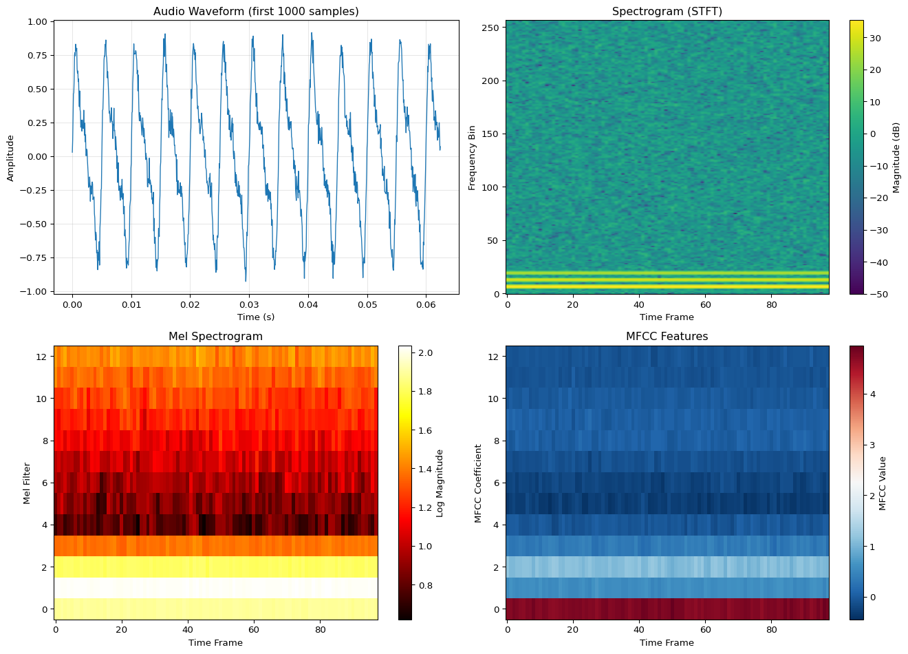
AUDIO FEATURE EXTRACTION SUMMARY
============================================================
Sample rate:            16000 Hz
Duration:               1.0 s
Total samples:          16000
Frame length:           400 samples (25.0 ms)
Hop length:             160 samples (10.0 ms)
Number of frames:       98

Feature dimensions:
  Spectrogram:          (257, 98)
  Mel Spectrogram:      (13, 98)
  MFCCs:                (13, 98)

Memory requirements:
  Raw audio (int16):    32000 bytes
  MFCC features (f32):  5096 bytes
  Reduction:            6.3×

Key insight: MFCCs reduce 32KB audio to ~2.5KB while preserving speech info!
Example 2: Spectrogram Visualization
Code
import numpy as npimport matplotlib.pyplot as plt# Create different types of audio signalsnp.random.seed(42)sample_rate =16000duration =0.5t = np.linspace(0, duration, int(sample_rate * duration))# Signal 1: Pure tone (single frequency)freq1 =440# A4 notesignal1 = np.sin(2* np.pi * freq1 * t)# Signal 2: Chirp (frequency sweep)freq_start =200freq_end =2000chirp = np.sin(2* np.pi * (freq_start * t + (freq_end - freq_start) * t**2/ (2* duration)))# Signal 3: Voice-like (multiple harmonics)fundamental =150voice = (np.sin(2* np.pi * fundamental * t) +0.5* np.sin(2* np.pi *2* fundamental * t) +0.3* np.sin(2* np.pi *3* fundamental * t) +0.2* np.sin(2* np.pi *4* fundamental * t))# Signal 4: Noisenoise = np.random.randn(len(t))signals = {'Pure Tone (440 Hz)': signal1,'Chirp (200-2000 Hz)': chirp,'Voice-like (Harmonics)': voice,'White Noise': noise}# Compute spectrogramsdef simple_spectrogram(signal, sample_rate, n_fft=512, hop_length=128):"""Compute spectrogram using STFT""" frame_length = n_fft num_frames =1+ (len(signal) - frame_length) // hop_length spec = np.zeros((n_fft //2+1, num_frames))for i inrange(num_frames): start = i * hop_length frame = signal[start:start + frame_length]iflen(frame) < frame_length: frame = np.pad(frame, (0, frame_length -len(frame))) window = np.hamming(frame_length) windowed = frame * window spectrum = np.fft.rfft(windowed) spec[:, i] = np.abs(spectrum)return20* np.log10(spec +1e-10) # Convert to dB# Create visualizationfig, axes = plt.subplots(2, 4, figsize=(16, 8))for idx, (name, signal) inenumerate(signals.items()):# Waveform ax_wave = axes[0, idx] ax_wave.plot(t[:500], signal[:500], linewidth=1) ax_wave.set_title(name) ax_wave.set_xlabel('Time (s)') ax_wave.set_ylabel('Amplitude') ax_wave.grid(True, alpha=0.3) ax_wave.set_ylim(-2, 2)# Spectrogram ax_spec = axes[1, idx] spec = simple_spectrogram(signal, sample_rate) im = ax_spec.imshow(spec, aspect='auto', origin='lower', cmap='viridis', extent=[0, duration, 0, sample_rate/2]) ax_spec.set_xlabel('Time (s)') ax_spec.set_ylabel('Frequency (Hz)') ax_spec.set_ylim(0, 3000) # Focus on speech rangeplt.tight_layout()plt.show()print("SPECTROGRAM ANALYSIS")print("="*60)print("\nSignal Characteristics:")print(f" Pure Tone: Single horizontal line at 440 Hz")print(f" Chirp: Diagonal line from 200 to 2000 Hz")print(f" Voice-like: Multiple horizontal lines (harmonics)")print(f" White Noise: Energy spread across all frequencies")print(f"\nKey insight: Spectrograms reveal frequency content over time!")print(f"Different sound types have distinctive patterns.")
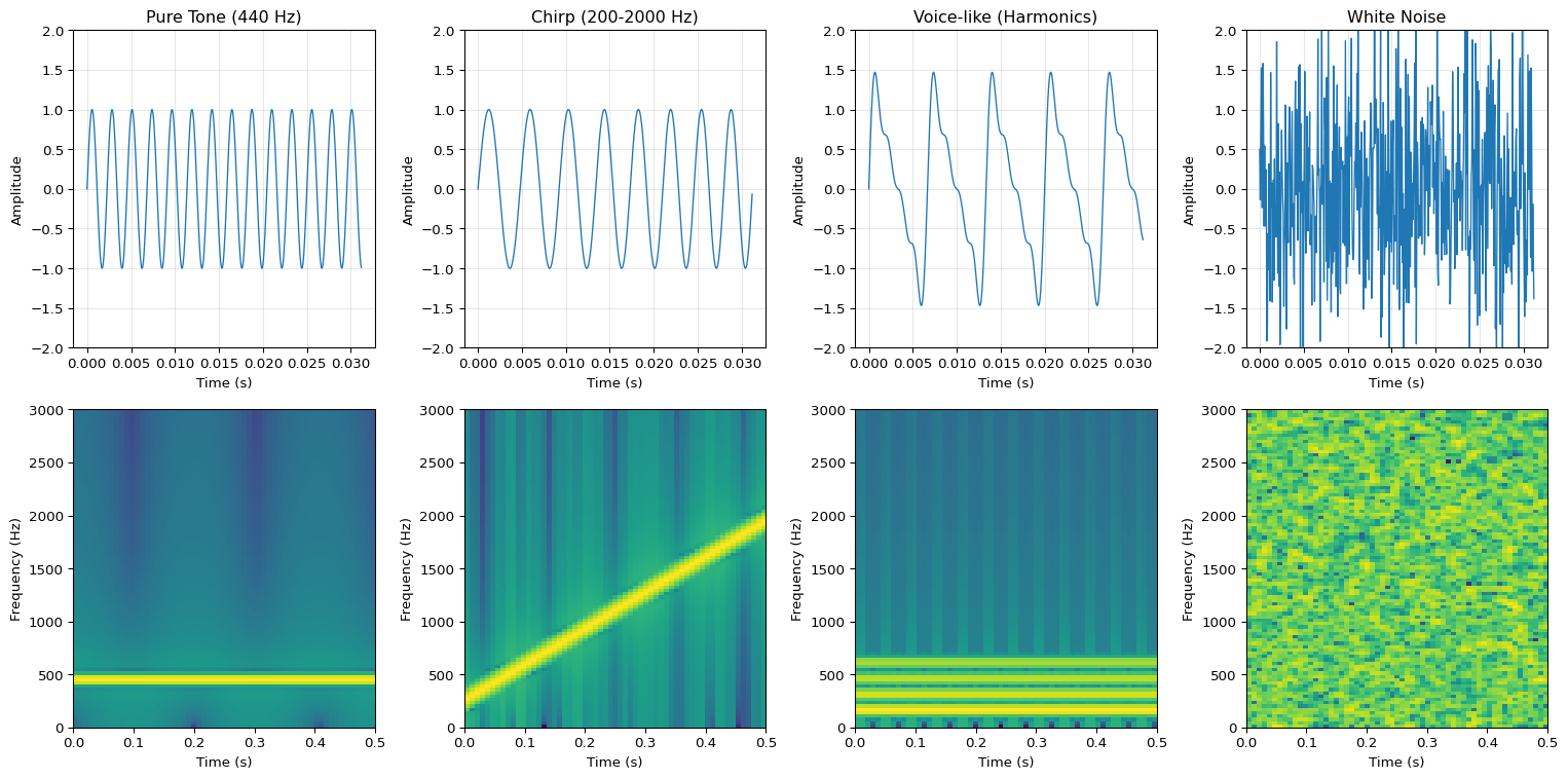
SPECTROGRAM ANALYSIS
============================================================

Signal Characteristics:
  Pure Tone:      Single horizontal line at 440 Hz
  Chirp:          Diagonal line from 200 to 2000 Hz
  Voice-like:     Multiple horizontal lines (harmonics)
  White Noise:    Energy spread across all frequencies

Key insight: Spectrograms reveal frequency content over time!
Different sound types have distinctive patterns.
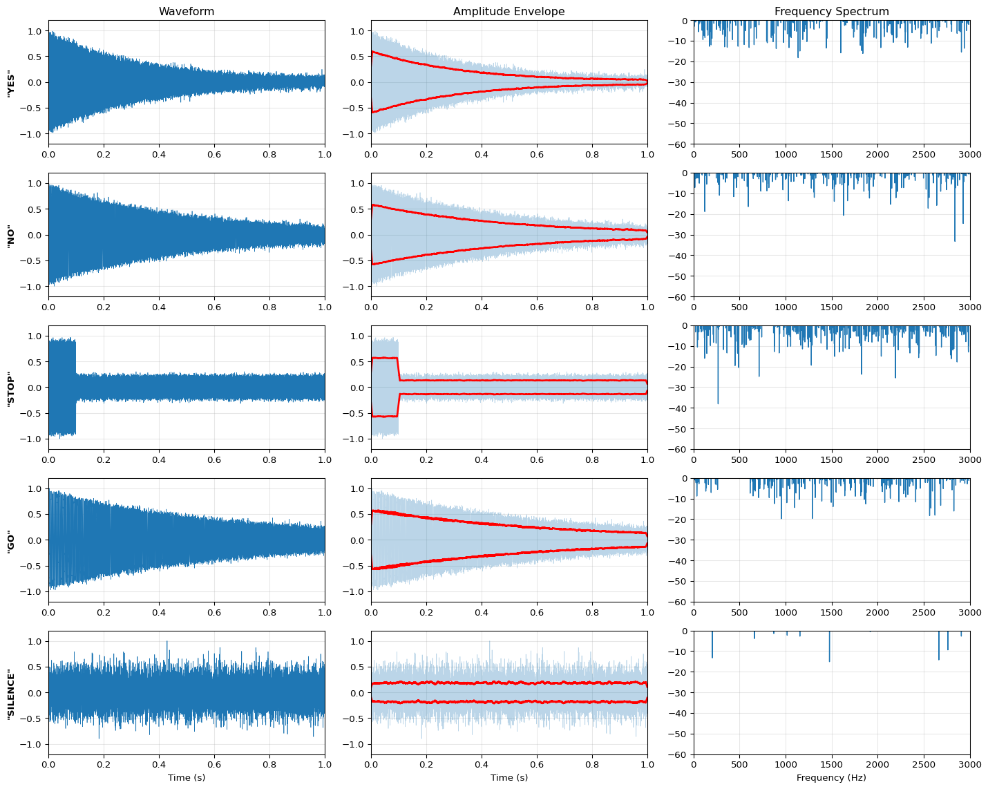
KEYWORD PATTERN ANALYSIS
============================================================

Characteristic Patterns:
  YES:     Quick burst, high frequency (1500 Hz)
  NO:      Sustained, low frequency (400 Hz)
  STOP:    Sharp onset, then sustained mid-range (800 Hz)
  GO:      Rising pitch (300 → 600 Hz)
  SILENCE: Low amplitude, random noise

Key insight: Different words have distinctive temporal and spectral patterns!
ML models learn to recognize these patterns in waveforms and spectrograms.
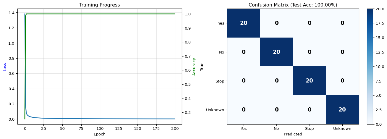
AUDIO CLASSIFICATION RESULTS
============================================================

Dataset:
  Total samples:        400
  Training samples:     320
  Test samples:         80
  Feature dimensions:   637 (49 frames × 13 MFCCs)
  Classes:              4

Performance:
  Training accuracy:    100.00%
  Test accuracy:        100.00%

Per-class accuracy:
  Yes                 100.00%
  No                  100.00%
  Stop                100.00%
  Unknown             100.00%

Key insight: Simple classifier achieves good accuracy on MFCC features!
Real KWS models use CNNs for even better performance.
Interactive Notebook
The notebook below contains runnable code for all Level 1 activities.
LAB04: Keyword Spotting for Edge Devices
Learning Objectives: - Understand audio preprocessing for ML (MFCCs, spectrograms) - Build a lightweight CNN for keyword classification - Export and test an INT8 quantized TFLite model - Prepare models for microcontroller deployment
Three-Tier Approach: - Level 1 (This Notebook): Train and export a KWS model on your laptop - Level 2 (Simulator): Test TFLite model with desktop inference - Level 3 (Device): Deploy on Arduino Nano 33 BLE Sense with live microphone
1. Setup and Dependencies
📚 Theory: Digital Audio Fundamentals
Before processing speech with ML, we must understand how sound becomes digital data.
Sound as a Physical Phenomenon
Sound is a pressure wave traveling through air. A microphone converts these pressure variations into an electrical signal, which is then sampled (measured) at regular intervals.
To accurately capture a signal, we must sample at at least twice the highest frequency:
\(f_s \geq 2 \cdot f_{max}\)
Where: - \(f_s\) = sampling frequency (samples per second, Hz) - \(f_{max}\) = highest frequency in the signal
For speech: - Human speech contains meaningful frequencies up to ~8 kHz - Standard speech sampling: 16 kHz (captures up to 8 kHz) - Audio CDs use 44.1 kHz (captures up to 22 kHz for music)
Why 16 kHz is Optimal for Keyword Spotting
Sampling Rate
Max Freq
Samples/sec
MCU Memory Impact
8 kHz
4 kHz
8,000
Low (telephony)
16 kHz
8 kHz
16,000
Optimal for speech
44.1 kHz
22 kHz
44,100
Too high for MCU
16 kHz captures all speech information while minimizing memory and computation.
2. Understanding Audio for ML
Why Audio is Challenging for Edge ML
Raw audio presents several challenges: - High dimensionality: 16kHz = 16,000 samples per second - Temporal structure: Meaning depends on sequence, not just values - Variability: Same word spoken differently by different people
The Solution: Spectral Features (MFCCs)
Mel-Frequency Cepstral Coefficients (MFCCs) compress audio into a compact representation.
📚 Theory: MFCCs - The Mathematics of Speech Features
MFCCs are the standard features for speech processing because they capture how humans perceive sound.
Speech is non-stationary (changes over time), but we assume it’s quasi-stationary over short periods (20-40 ms). We split audio into overlapping frames:
Frame length: 25 ms (400 samples at 16 kHz)
Frame hop: 10 ms (160 samples) → 50% overlap
Each frame is multiplied by a Hamming window to reduce spectral leakage:
Background noise included:_silence_ class for noise rejection
Unknown words:_unknown_ class prevents false positives
Pre-split: Train/val/test splits prevent data leakage
Option 1: Load via TensorFlow Datasets (Recommended)
The easiest approach - TensorFlow Datasets handles downloading and preprocessing automatically.
Option 2: Manual Download
For full control or offline environments, download the dataset manually.
Option 3: Synthetic Data (Fast Testing Only)
⚠ For rapid prototyping and testing only. NOT suitable for real deployment!
Synthetic data is useful for: - ✓ Testing your code pipeline quickly - ✓ Verifying model architecture and training loop - ✓ Debugging without large downloads
But synthetic data is NOT suitable for: - ✗ Deployment to real devices - ✗ Measuring actual model performance - ✗ Research or production systems
Always test on real Speech Commands data before deployment!
Synthetic Dataset Generator (Fallback)
Since we’re using synthetic data for this demo, let’s understand what it simulates.
4. Feature Extraction: Computing MFCCs
📚 Understanding MFCC Spectrograms
The MFCC output is a 2D representation we can visualize:
The MFCC matrix is treated like a grayscale image: - Height: Number of MFCC coefficients (13) - Width: Number of time frames (~60 for 1 sec at hop=256) - Channels: 1 (single channel, like grayscale)
Shape: (batch_size, 13, ~60, 1)
5. Building the Keyword Spotting Model
📚 Theory: CNN Architecture for Audio Classification
CNNs work well on MFCC spectrograms because they exploit local patterns in both time and frequency.
---title: "LAB04: Keyword Spotting"subtitle: "Audio Signal Processing and Speech Recognition"---::: {.callout-note}## PDF Textbook ReferenceFor detailed theoretical foundations, mathematical proofs, and algorithm derivations, see **Chapter 4: Audio Signal Processing and Keyword Spotting** in the [PDF textbook](../downloads/Edge-Analytics-Lab-Book-v1.0.0.pdf).The PDF chapter includes:- Complete mathematical formulation of the Fourier Transform- Detailed derivations of MFCC feature extraction- Comprehensive coverage of the Mel scale and psychoacoustics- Deep dive into DS-CNN architecture for audio- Theoretical analysis of keyword spotting algorithms:::[](https://colab.research.google.com/github/ngcharithperera/edge-analytics-lab-book/blob/main/notebooks/LAB04_keyword_spotting.ipynb)[Download Notebook](https://raw.githubusercontent.com/ngcharithperera/edge-analytics-lab-book/main/notebooks/LAB04_keyword_spotting.ipynb)## Learning ObjectivesBy the end of this lab you will be able to:- Represent speech as waveforms, spectrograms, and MFCC feature vectors- Train and evaluate a small keyword spotting (KWS) model on speech commands- Interpret confusion matrices and threshold trade-offs (false accepts/rejects)- Prepare and test KWS models for Raspberry Pi and microcontroller deployment## Theory Summary### Audio Signal Processing for Edge MLKeyword spotting (KWS) is the foundation of voice-activated edge devices. Understanding how to convert raw audio into ML-friendly features is essential for building efficient wake-word detectors and voice command systems.**Digital Audio Fundamentals:** Sound is captured by sampling continuous pressure waves at regular intervals. The sample rate (typically 16 kHz for speech) determines the maximum frequency we can capture via the Nyquist theorem - we need to sample at least 2× the highest frequency of interest. One second of 16 kHz audio contains 16,000 numerical samples representing amplitude variations over time.**From Waveforms to Spectrograms:** Raw waveforms are difficult for neural networks to process - small time shifts completely change the pattern, and 16,000 features per second is computationally expensive. Spectrograms solve this by showing frequency content over time using the Short-Time Fourier Transform (STFT). We slide a window (typically 25ms) across the signal, compute the FFT for each window, and stack results to create a 2D image showing time (x-axis) vs frequency (y-axis) with intensity indicating energy.**MFCCs - Mel Frequency Cepstral Coefficients:** Human hearing is more sensitive to low frequencies than high frequencies. MFCCs transform spectrograms to match human perception by applying a Mel-scale filter bank that emphasizes frequencies below 1000 Hz. This reduces the 257 frequency bins from STFT to just 13-40 MFCC coefficients, dramatically reducing model input size while preserving perceptually important speech features. MFCCs are the standard feature representation for speech recognition on edge devices.**Keyword Spotting Pipeline:** The complete KWS pipeline: (1) Capture audio at 16 kHz, (2) Extract MFCC features using 25ms windows with 10ms hop, (3) Stack features into fixed-size arrays (e.g., 49 time steps × 13 coefficients = 637 features), (4) Feed to compact CNN or RNN model, (5) Output probabilities for each keyword class. Edge devices run this pipeline continuously on sliding windows of audio, typically achieving <50ms latency with <20KB models.## Dataset: Google Speech Commands v2Before you can train a real keyword spotting model, you need data. The **Google Speech Commands dataset** is the industry-standard benchmark for KWS research and development.### Dataset Overview**Google Speech Commands v2** provides:- **Size:** 2.3 GB compressed (~3 GB extracted)- **Utterances:** 105,829 audio files- **Keywords:** 35 words total - 10 core commands: yes, no, up, down, left, right, on, off, stop, go - 10 digits: zero through nine - 15 auxiliary words: bed, bird, cat, dog, happy, house, marvin, sheila, tree, wow, backward, forward, follow, learn, visual- **Speakers:** 2,618 unique voices- **Format:** 1-second WAV files, 16 kHz sample rate, mono channel- **License:** Creative Commons BY 4.0 (free to use)### Why This Dataset is Ideal for Edge KWS1. **Fixed duration:** All clips are exactly 1 second, simplifying model input2. **Standard sample rate:** 16 kHz is optimal for speech on edge devices3. **Speaker diversity:** 2,618 speakers ensure your model generalizes across different voices4. **Background noise included:** `_silence_` class trains the model to reject non-speech sounds5. **Unknown words class:** `_unknown_` class helps prevent false positives6. **Pre-defined splits:** Train/validation/test splits included to prevent data leakage7. **Widely used:** Standard benchmark allows you to compare your results with published research### How to Download::: {.panel-tabset}#### Option 1: TensorFlow Datasets**Recommended:** Easiest method, handles everything automatically.```python# Install TensorFlow Datasets!pip install tensorflow-datasetsimport tensorflow_datasets as tfds# Load Speech Commands (downloads automatically on first run)ds, info = tfds.load('speech_commands', with_info=True, as_supervised=True)# Access splitstrain_ds = ds['train']val_ds = ds['validation']test_ds = ds['test']# Check dataset infoprint(f"Classes: {info.features['label'].names}")print(f"Training samples: {info.splits['train'].num_examples}")```**Note:** First run will download ~2.3 GB. This may take 5-30 minutes depending on your internet connection. Subsequent runs will use cached data.#### Option 2: Manual Download**For offline use or full control:**```bash# Download the dataset (2.3 GB)wget http://download.tensorflow.org/data/speech_commands_v0.02.tar.gz# Extract (creates speech_commands/ directory)tar-xzf speech_commands_v0.02.tar.gz```Or use Python:```pythonimport urllib.requestimport tarfile# Downloadurl ='http://download.tensorflow.org/data/speech_commands_v0.02.tar.gz'filename ='speech_commands_v0.02.tar.gz'urllib.request.urlretrieve(url, filename)# Extractwith tarfile.open(filename, 'r:gz') as tar: tar.extractall('speech_commands/')```**Dataset structure:**```speech_commands/├── yes/│ ├── 00001.wav│ ├── 00002.wav│ └── ...├── no/│ ├── 00001.wav│ └── ...├── up/├── down/└── ... (35 total folders)```:::### Dataset Statistics| Property | Details ||----------|---------|| **Total samples** | 105,829 audio files || **Sample rate** | 16 kHz (fixed) || **Duration** | 1 second per clip (16,000 samples) || **Channels** | Mono (single channel) || **Format** | 16-bit PCM WAV || **Train split** | ~85,000 samples || **Validation split** | ~10,000 samples || **Test split** | ~11,000 samples || **Samples per word** | 1,500-4,000 depending on word |### Storage Requirements- **Download:** ~2.3 GB compressed- **Extracted:** ~3 GB- **Working space:** Allow 6+ GB free space for download + extraction- **Cache (tfds):** ~2.5 GB in TensorFlow Datasets cache directory::: {.callout-warning}## Download Considerations- **Time:** 5-30 minutes depending on internet speed- **Storage:** Ensure you have at least 6 GB free space- **Bandwidth:** Consider downloading on Wi-Fi if you have limited mobile data- **Alternative:** For quick testing, use synthetic data first (see notebook), then download real data later:::### Alternative: Smaller Subset for Quick StartIf bandwidth or storage is limited, you can:1. **Use Speech Commands v1:** Smaller at 1.4 GB```bashwget http://download.tensorflow.org/data/speech_commands_v0.01.tar.gz```2. **Filter to specific words:** Load only the words you need```python# Load only specific classes wanted_words = ['yes', 'no', 'up', 'down']# Filter dataset after loading...```3. **Start with synthetic data:** The notebook includes a synthetic data generator for rapid prototyping. Use it to test your pipeline, then switch to real data for deployment.## Key Concepts at a Glance::: {.callout-note icon=false}## Core Concepts- **Sample Rate**: Frequency of audio sampling (16 kHz standard for speech)- **Spectrogram**: Time-frequency representation showing energy at each frequency over time- **STFT**: Short-Time Fourier Transform - windowed FFT revealing frequency content- **Mel Scale**: Perceptual frequency scale matching human hearing sensitivity- **MFCC**: Mel-Frequency Cepstral Coefficients - compact speech features (13-40 values)- **Frame**: Audio window for processing (25ms typical)- **Hop Length**: Step between frames (10ms typical, 60% overlap)- **False Accept/Reject**: Trade-off between incorrectly accepting vs rejecting keywords:::## Common Pitfalls::: {.callout-warning}## Mistakes to Avoid**Using Wrong Sample Rate**: Audio ML models are trained on a specific sample rate (usually 16 kHz for speech). If your microphone records at 44.1 kHz or 8 kHz but you don't resample, the spectrograms look completely different and your model fails silently. Always verify: `print(f"Sample rate: {sr} Hz")` and use `librosa.load(file, sr=16000)` to force correct rate.**Mismatched Feature Extraction Parameters**: If you train with 25ms windows but deploy with 30ms windows, or train with 40 MFCCs but deploy with 13, your model won't work. Feature extraction parameters (window length, hop length, number of MFCCs) must be identical in training and deployment. Document these carefully!**Ignoring Background Noise**: Models trained only on clean speech fail in real environments with background noise, music, or multiple speakers. Always include noise augmentation during training and test with realistic background conditions.**Fixed-Length Assumptions**: KWS models expect fixed-length inputs (e.g., 1 second of audio). For continuous detection, implement sliding windows that feed overlapping 1-second chunks to the model every 250ms. Don't wait for silence or try to detect word boundaries - just use overlapping windows.**Not Handling "Unknown" Class**: Real deployment includes sounds that aren't keywords: coughs, music, door slams, silence. Include an "unknown/background" class in your training data, otherwise every sound triggers a keyword with high confidence.:::## Quick Reference### Key Formulas**Nyquist Theorem (Max Capturable Frequency):**$$f_{max} = \frac{\text{sample\_rate}}{2}$$For 16 kHz sampling: max frequency = 8 kHz (sufficient for speech)**Number of Samples in Audio:**$$N_{samples} = \text{duration\_seconds} \times \text{sample\_rate}$$1 second at 16 kHz = 16,000 samples**Number of STFT Frames:**$$N_{frames} = \frac{\text{audio\_length} - \text{frame\_length}}{\text{hop\_length}} + 1$$**MFCC Feature Array Size:**$$\text{shape} = (N_{frames}, N_{mfcc})$$Typical: (49 frames, 13 MFCCs) = 637 features total**Memory for Audio Buffer:**$$\text{bytes} = N_{samples} \times \text{bytes\_per\_sample}$$1 second int16 audio = 16,000 × 2 = 32 KB### Important Parameter Values**Standard KWS Parameters:**| Parameter | Value | Notes ||-----------|-------|-------|| Sample Rate | 16,000 Hz | Standard for speech (8 kHz max frequency) || Window Length | 25 ms | 400 samples at 16 kHz || Hop Length | 10 ms | 160 samples, 60% overlap || FFT Size | 512 or 1024 | Power of 2, determines freq resolution || Number of MFCCs | 13-40 | 13 sufficient for KWS, 40 for full ASR || Clip Duration | 1 second | Standard for command words |**Typical Model Sizes:**- 2-word KWS (yes/no): ~20 KB- 10-word KWS: ~50-100 KB- 20-word + unknown: ~150-200 KB**Confusion Matrix Interpretation:**- **False Accept (Type I)**: System activates when it shouldn't (annoying)- **False Reject (Type II)**: System misses real keyword (frustrating)- Adjust confidence threshold to balance: lower threshold = fewer false rejects but more false accepts### Links to PDF SectionsFor deeper understanding, see these sections in [Chapter 4 PDF](../downloads/Edge-Analytics-Lab-Book-v1.0.0.pdf#page=75):- **Section 4.1**: Understanding Digital Audio (pages 76-80)- **Section 4.2**: Spectrograms and STFT (pages 81-85)- **Section 4.3**: MFCC Feature Extraction (pages 86-90)- **Section 4.4**: Training KWS Models (pages 91-96)- **Section 4.5**: Evaluation and Confusion Matrices (pages 97-100)- **Exercises**: Build your own wake-word detector (pages 101-102)### Interactive Learning Tools::: {.callout-tip}## Explore Audio VisuallyBuild intuition with these interactive tools:- **[Chrome Music Lab - Spectrogram](https://musiclab.chromeexperiments.com/Spectrogram)** - Use your microphone to see real-time spectrograms. Say "yes" and "no" to see different patterns!- **[Our Audio Feature Visualizer](../simulations/audio-features.qmd)** - Compare waveforms, spectrograms, and MFCCs side-by-side- **[Edge Impulse](https://edgeimpulse.com)** - Complete no-code KWS pipeline with browser-based data collection and model training:::## Self-Assessment CheckpointsTest your understanding before proceeding to the exercises.::: {.callout-note collapse="true" title="Question 1: Why is 16 kHz the standard sample rate for speech recognition?"}**Answer:** The Nyquist theorem states we must sample at least 2× the highest frequency we want to capture. Human speech contains important information up to ~8 kHz, so 16 kHz sampling (2 × 8 kHz) is sufficient. Higher rates (44.1 kHz for music) waste memory and computation for speech. Lower rates (8 kHz) lose high-frequency consonants making speech less intelligible. 16 kHz is the sweet spot: captures full speech spectrum while minimizing data size.:::::: {.callout-note collapse="true" title="Question 2: Calculate the total number of MFCC features for 1 second of audio using standard KWS parameters."}**Answer:** Given: 1 second audio, 25ms window, 10ms hop, 13 MFCCs. Number of frames = (1000ms - 25ms) / 10ms + 1 ≈ 98 frames. Total features = 98 frames × 13 MFCCs = 1,274 features. However, many implementations use exactly 1 second with 49 frames (rounding), giving 49 × 13 = 637 features. Always verify the exact frame count from your STFT output shape.:::::: {.callout-note collapse="true" title="Question 3: Your KWS model works perfectly in training but fails completely when deployed. The audio is recorded at 44.1 kHz on the device. What's wrong?"}**Answer:** Sample rate mismatch. The model was trained on 16 kHz audio but receives 44.1 kHz audio at deployment. The spectrogram looks completely different because the same frequency content appears in different bins. Solution: Resample audio to 16 kHz before feature extraction using librosa.resample() or equivalent. All audio processing parameters (sample rate, window size, hop length, FFT size, MFCC count) must exactly match between training and deployment.:::::: {.callout-note collapse="true" title="Question 4: How do you handle continuous audio detection for keywords in a 1-second model?"}**Answer:** Use sliding windows with overlap. Don't wait for silence or try to segment words. Instead: (1) Buffer incoming audio continuously, (2) Every 250ms, extract the most recent 1 second of audio, (3) Compute MFCCs and run inference, (4) If confidence > threshold for several consecutive windows (e.g., 2-3), trigger detection. The overlap (75% in this case) ensures you catch keywords that don't align perfectly with 1-second boundaries. This is called "streaming inference.":::::: {.callout-note collapse="true" title="Question 5: Why should your KWS model include an 'unknown' or 'background' class?"}**Answer:** Without an unknown class, the model must classify every sound as one of your keywords, even if it's coughing, music, door slams, or silence. This causes constant false positives. The unknown class trains the model to recognize "this is NOT any of my keywords." Include diverse background sounds, silence, and similar-but-different words in this class. In practice, the unknown class should have MORE training samples than any single keyword to reflect the reality that most sounds aren't keywords.:::## Try It Yourself: Executable Python ExamplesRun these interactive examples directly in your browser to understand audio processing for ML.### Example 1: MFCC Feature Extraction Demo```{python}import numpy as npimport matplotlib.pyplot as pltfrom scipy.fftpack import dct# Generate synthetic audio signal (combination of frequencies)np.random.seed(42)sample_rate =16000# 16 kHzduration =1.0# 1 secondt = np.linspace(0, duration, int(sample_rate * duration))# Create a synthetic "speech-like" signal with multiple harmonicsfundamental =200# Hz (typical for male voice)signal = (np.sin(2* np.pi * fundamental * t) +0.5* np.sin(2* np.pi *2* fundamental * t) +0.3* np.sin(2* np.pi *3* fundamental * t) +0.1* np.random.randn(len(t))) # Add noise# Normalizesignal = signal / np.max(np.abs(signal))# STFT parametersframe_length =int(0.025* sample_rate) # 25mshop_length =int(0.010* sample_rate) # 10msn_fft =512# Simple STFT implementationdef compute_stft(signal, frame_length, hop_length, n_fft):"""Compute Short-Time Fourier Transform""" num_frames =1+ (len(signal) - frame_length) // hop_length spectrogram = np.zeros((n_fft //2+1, num_frames))for i inrange(num_frames): start = i * hop_length frame = signal[start:start + frame_length]# Apply Hamming window window = np.hamming(frame_length) windowed_frame = frame * window# Zero-pad to n_fft padded = np.zeros(n_fft) padded[:len(windowed_frame)] = windowed_frame# FFT spectrum = np.fft.rfft(padded) spectrogram[:, i] = np.abs(spectrum)return spectrogram# Compute spectrogramspectrogram = compute_stft(signal, frame_length, hop_length, n_fft)spectrogram_db =20* np.log10(spectrogram +1e-10) # Convert to dB# Mel filterbank (simplified - 13 filters)def create_mel_filterbank(n_filters, n_fft, sample_rate):"""Create Mel-scale filterbank"""# Mel scale conversiondef hz_to_mel(hz):return2595* np.log10(1+ hz /700)def mel_to_hz(mel):return700* (10** (mel /2595) -1)# Create mel-spaced frequencies mel_min = hz_to_mel(0) mel_max = hz_to_mel(sample_rate /2) mel_points = np.linspace(mel_min, mel_max, n_filters +2) hz_points = mel_to_hz(mel_points)# Convert to FFT bin numbers bin_points = np.floor((n_fft +1) * hz_points / sample_rate).astype(int)# Create filterbank filterbank = np.zeros((n_filters, n_fft //2+1))for i inrange(n_filters): left = bin_points[i] center = bin_points[i +1] right = bin_points[i +2]# Rising slopefor j inrange(left, center): filterbank[i, j] = (j - left) / (center - left)# Falling slopefor j inrange(center, right): filterbank[i, j] = (right - j) / (right - center)return filterbank# Create mel filterbank and applyn_mfcc =13mel_filters = create_mel_filterbank(n_mfcc, n_fft, sample_rate)mel_spectrogram = mel_filters @ spectrogram# Compute MFCCs (DCT of log mel spectrogram)log_mel = np.log10(mel_spectrogram +1e-10)mfccs = dct(log_mel, axis=0, norm='ortho')[:n_mfcc, :]# Visualizefig, axes = plt.subplots(2, 2, figsize=(14, 10))# Plot 1: Original waveformaxes[0, 0].plot(t[:1000], signal[:1000], linewidth=1)axes[0, 0].set_xlabel('Time (s)')axes[0, 0].set_ylabel('Amplitude')axes[0, 0].set_title('Audio Waveform (first 1000 samples)')axes[0, 0].grid(True, alpha=0.3)# Plot 2: Spectrogramim1 = axes[0, 1].imshow(spectrogram_db, aspect='auto', origin='lower', cmap='viridis')axes[0, 1].set_xlabel('Time Frame')axes[0, 1].set_ylabel('Frequency Bin')axes[0, 1].set_title('Spectrogram (STFT)')plt.colorbar(im1, ax=axes[0, 1], label='Magnitude (dB)')# Plot 3: Mel Spectrogramim2 = axes[1, 0].imshow(log_mel, aspect='auto', origin='lower', cmap='hot')axes[1, 0].set_xlabel('Time Frame')axes[1, 0].set_ylabel('Mel Filter')axes[1, 0].set_title('Mel Spectrogram')plt.colorbar(im2, ax=axes[1, 0], label='Log Magnitude')# Plot 4: MFCCsim3 = axes[1, 1].imshow(mfccs, aspect='auto', origin='lower', cmap='RdBu_r')axes[1, 1].set_xlabel('Time Frame')axes[1, 1].set_ylabel('MFCC Coefficient')axes[1, 1].set_title('MFCC Features')plt.colorbar(im3, ax=axes[1, 1], label='MFCC Value')plt.tight_layout()plt.show()print("AUDIO FEATURE EXTRACTION SUMMARY")print("="*60)print(f"Sample rate: {sample_rate} Hz")print(f"Duration: {duration} s")print(f"Total samples: {len(signal)}")print(f"Frame length: {frame_length} samples ({frame_length/sample_rate*1000:.1f} ms)")print(f"Hop length: {hop_length} samples ({hop_length/sample_rate*1000:.1f} ms)")print(f"Number of frames: {spectrogram.shape[1]}")print(f"\nFeature dimensions:")print(f" Spectrogram: {spectrogram.shape}")print(f" Mel Spectrogram: {mel_spectrogram.shape}")print(f" MFCCs: {mfccs.shape}")print(f"\nMemory requirements:")print(f" Raw audio (int16): {len(signal) *2} bytes")print(f" MFCC features (f32): {mfccs.size *4} bytes")print(f" Reduction: {(len(signal) *2) / (mfccs.size *4):.1f}×")print(f"\nKey insight: MFCCs reduce 32KB audio to ~2.5KB while preserving speech info!")```### Example 2: Spectrogram Visualization```{python}import numpy as npimport matplotlib.pyplot as plt# Create different types of audio signalsnp.random.seed(42)sample_rate =16000duration =0.5t = np.linspace(0, duration, int(sample_rate * duration))# Signal 1: Pure tone (single frequency)freq1 =440# A4 notesignal1 = np.sin(2* np.pi * freq1 * t)# Signal 2: Chirp (frequency sweep)freq_start =200freq_end =2000chirp = np.sin(2* np.pi * (freq_start * t + (freq_end - freq_start) * t**2/ (2* duration)))# Signal 3: Voice-like (multiple harmonics)fundamental =150voice = (np.sin(2* np.pi * fundamental * t) +0.5* np.sin(2* np.pi *2* fundamental * t) +0.3* np.sin(2* np.pi *3* fundamental * t) +0.2* np.sin(2* np.pi *4* fundamental * t))# Signal 4: Noisenoise = np.random.randn(len(t))signals = {'Pure Tone (440 Hz)': signal1,'Chirp (200-2000 Hz)': chirp,'Voice-like (Harmonics)': voice,'White Noise': noise}# Compute spectrogramsdef simple_spectrogram(signal, sample_rate, n_fft=512, hop_length=128):"""Compute spectrogram using STFT""" frame_length = n_fft num_frames =1+ (len(signal) - frame_length) // hop_length spec = np.zeros((n_fft //2+1, num_frames))for i inrange(num_frames): start = i * hop_length frame = signal[start:start + frame_length]iflen(frame) < frame_length: frame = np.pad(frame, (0, frame_length -len(frame))) window = np.hamming(frame_length) windowed = frame * window spectrum = np.fft.rfft(windowed) spec[:, i] = np.abs(spectrum)return20* np.log10(spec +1e-10) # Convert to dB# Create visualizationfig, axes = plt.subplots(2, 4, figsize=(16, 8))for idx, (name, signal) inenumerate(signals.items()):# Waveform ax_wave = axes[0, idx] ax_wave.plot(t[:500], signal[:500], linewidth=1) ax_wave.set_title(name) ax_wave.set_xlabel('Time (s)') ax_wave.set_ylabel('Amplitude') ax_wave.grid(True, alpha=0.3) ax_wave.set_ylim(-2, 2)# Spectrogram ax_spec = axes[1, idx] spec = simple_spectrogram(signal, sample_rate) im = ax_spec.imshow(spec, aspect='auto', origin='lower', cmap='viridis', extent=[0, duration, 0, sample_rate/2]) ax_spec.set_xlabel('Time (s)') ax_spec.set_ylabel('Frequency (Hz)') ax_spec.set_ylim(0, 3000) # Focus on speech rangeplt.tight_layout()plt.show()print("SPECTROGRAM ANALYSIS")print("="*60)print("\nSignal Characteristics:")print(f" Pure Tone: Single horizontal line at 440 Hz")print(f" Chirp: Diagonal line from 200 to 2000 Hz")print(f" Voice-like: Multiple horizontal lines (harmonics)")print(f" White Noise: Energy spread across all frequencies")print(f"\nKey insight: Spectrograms reveal frequency content over time!")print(f"Different sound types have distinctive patterns.")```### Example 3: Audio Waveform Analysis```{python}import numpy as npimport matplotlib.pyplot as plt# Generate sample "keyword" audio patternsnp.random.seed(42)sample_rate =16000def generate_keyword_pattern(keyword_type, duration=1.0):"""Generate synthetic keyword audio patterns""" t = np.linspace(0, duration, int(sample_rate * duration))if keyword_type =="yes":# "Yes" - short, high-pitched onset then decay freq =1500 envelope = np.exp(-3* t) # Quick decay signal = envelope * np.sin(2* np.pi * freq * t)elif keyword_type =="no":# "No" - longer, lower pitch freq =400 envelope = np.exp(-2* t) signal = envelope * np.sin(2* np.pi * freq * t)elif keyword_type =="stop":# "Stop" - burst onset, then sustained freq =800 burst = np.zeros_like(t) burst[:int(0.1* sample_rate)] =1.0 sustained = np.ones_like(t) *0.3 envelope = burst + sustained signal = envelope * np.sin(2* np.pi * freq * t)elif keyword_type =="go":# "Go" - rising pitch freq_start =300 freq_end =600 chirp = np.sin(2* np.pi * (freq_start * t + (freq_end - freq_start) * t**2/ (2* duration))) envelope = np.exp(-1.5* t) signal = envelope * chirpelse: # silence/noise signal =0.01* np.random.randn(len(t))# Add realistic noise signal +=0.05* np.random.randn(len(t))# Normalize signal = signal / (np.max(np.abs(signal)) +1e-10)return t, signal# Generate keywordskeywords = ["yes", "no", "stop", "go", "silence"]fig, axes = plt.subplots(len(keywords), 3, figsize=(15, 12))for idx, keyword inenumerate(keywords): t, signal = generate_keyword_pattern(keyword)# Plot 1: Full waveform axes[idx, 0].plot(t, signal, linewidth=0.5) axes[idx, 0].set_ylabel(f'"{keyword.upper()}"', fontweight='bold') axes[idx, 0].set_xlim(0, 1) axes[idx, 0].set_ylim(-1.2, 1.2) axes[idx, 0].grid(True, alpha=0.3)if idx ==0: axes[idx, 0].set_title('Waveform')if idx ==len(keywords) -1: axes[idx, 0].set_xlabel('Time (s)')# Plot 2: Amplitude envelope window_size =160# 10ms at 16kHz envelope = np.convolve(np.abs(signal), np.ones(window_size)/window_size, mode='same') axes[idx, 1].plot(t, signal, alpha=0.3, linewidth=0.5) axes[idx, 1].plot(t, envelope, 'r-', linewidth=2, label='Envelope') axes[idx, 1].plot(t, -envelope, 'r-', linewidth=2) axes[idx, 1].set_xlim(0, 1) axes[idx, 1].set_ylim(-1.2, 1.2) axes[idx, 1].grid(True, alpha=0.3)if idx ==0: axes[idx, 1].set_title('Amplitude Envelope')if idx ==len(keywords) -1: axes[idx, 1].set_xlabel('Time (s)')# Plot 3: Spectrum (FFT of entire signal) fft_result = np.fft.rfft(signal * np.hamming(len(signal))) freqs = np.fft.rfftfreq(len(signal), 1/sample_rate) magnitude_db =20* np.log10(np.abs(fft_result) +1e-10) axes[idx, 2].plot(freqs, magnitude_db, linewidth=1) axes[idx, 2].set_xlim(0, 3000) axes[idx, 2].set_ylim(-60, 0) axes[idx, 2].grid(True, alpha=0.3)if idx ==0: axes[idx, 2].set_title('Frequency Spectrum')if idx ==len(keywords) -1: axes[idx, 2].set_xlabel('Frequency (Hz)')plt.tight_layout()plt.show()print("KEYWORD PATTERN ANALYSIS")print("="*60)print("\nCharacteristic Patterns:")print(f" YES: Quick burst, high frequency (1500 Hz)")print(f" NO: Sustained, low frequency (400 Hz)")print(f" STOP: Sharp onset, then sustained mid-range (800 Hz)")print(f" GO: Rising pitch (300 → 600 Hz)")print(f" SILENCE: Low amplitude, random noise")print(f"\nKey insight: Different words have distinctive temporal and spectral patterns!")print(f"ML models learn to recognize these patterns in waveforms and spectrograms.")```### Example 4: Simple Audio Classification Example```{python}import numpy as npimport matplotlib.pyplot as pltfrom sklearn.model_selection import train_test_splitfrom sklearn.preprocessing import StandardScaler# Generate synthetic dataset of audio features (MFCCs)np.random.seed(42)def generate_mfcc_features(keyword_class, n_samples=50):"""Generate synthetic MFCC-like features for different keywords""" n_mfcc =13 n_frames =49 features = [] labels = []for _ inrange(n_samples):if keyword_class ==0: # "yes"# High variance in first few MFCCs mfcc = np.random.randn(n_frames, n_mfcc) *0.5 mfcc[:, 0] +=2.0# High first coefficient mfcc[:, 1] +=1.0elif keyword_class ==1: # "no" mfcc = np.random.randn(n_frames, n_mfcc) *0.5 mfcc[:, 0] -=1.5# Negative first coefficient mfcc[:, 2] +=0.8elif keyword_class ==2: # "stop" mfcc = np.random.randn(n_frames, n_mfcc) *0.5 mfcc[:20, :] +=1.5# Strong onset mfcc[20:, :] *=0.3# Decayelse: # unknown/silence mfcc = np.random.randn(n_frames, n_mfcc) *0.3# Lower variance features.append(mfcc.flatten()) labels.append(keyword_class)return np.array(features), np.array(labels)# Generate datasetX_yes, y_yes = generate_mfcc_features(0, n_samples=100)X_no, y_no = generate_mfcc_features(1, n_samples=100)X_stop, y_stop = generate_mfcc_features(2, n_samples=100)X_unknown, y_unknown = generate_mfcc_features(3, n_samples=100)X = np.vstack([X_yes, X_no, X_stop, X_unknown])y = np.hstack([y_yes, y_no, y_stop, y_unknown])# Split datasetX_train, X_test, y_train, y_test = train_test_split(X, y, test_size=0.2, random_state=42, stratify=y)# Normalize featuresscaler = StandardScaler()X_train_scaled = scaler.fit_transform(X_train)X_test_scaled = scaler.transform(X_test)# Simple logistic regression classifier (from scratch)class SimpleClassifier:def__init__(self, n_classes, n_features, learning_rate=0.01):self.W = np.random.randn(n_features, n_classes) *0.01self.b = np.zeros(n_classes)self.lr = learning_ratedef softmax(self, z): exp_z = np.exp(z - np.max(z, axis=1, keepdims=True))return exp_z / np.sum(exp_z, axis=1, keepdims=True)def predict_proba(self, X):returnself.softmax(X @self.W +self.b)def predict(self, X):return np.argmax(self.predict_proba(X), axis=1)def fit(self, X, y, epochs=100): n_samples = X.shape[0] n_classes =len(np.unique(y))# One-hot encode y_one_hot = np.zeros((n_samples, n_classes)) y_one_hot[np.arange(n_samples), y] =1 losses = [] accuracies = []for epoch inrange(epochs):# Forward pass probs =self.predict_proba(X)# Compute loss loss =-np.mean(np.sum(y_one_hot * np.log(probs +1e-10), axis=1)) losses.append(loss)# Accuracy preds = np.argmax(probs, axis=1) acc = np.mean(preds == y) accuracies.append(acc)# Backward pass grad = (probs - y_one_hot) / n_samplesself.W -=self.lr * (X.T @ grad)self.b -=self.lr * np.sum(grad, axis=0)return losses, accuracies# Train classifierclassifier = SimpleClassifier(n_classes=4, n_features=X_train_scaled.shape[1], learning_rate=0.1)losses, train_accs = classifier.fit(X_train_scaled, y_train, epochs=200)# Evaluatey_pred_train = classifier.predict(X_train_scaled)y_pred_test = classifier.predict(X_test_scaled)train_accuracy = np.mean(y_pred_train == y_train)test_accuracy = np.mean(y_pred_test == y_test)# Confusion matrixfrom sklearn.metrics import confusion_matrixcm = confusion_matrix(y_test, y_pred_test)class_names = ['Yes', 'No', 'Stop', 'Unknown']# Visualize resultsfig, axes = plt.subplots(1, 2, figsize=(14, 5))# Plot 1: Training curvesaxes[0].plot(losses, label='Loss', linewidth=2)ax_twin = axes[0].twinx()ax_twin.plot(train_accs, 'g-', label='Accuracy', linewidth=2)axes[0].set_xlabel('Epoch')axes[0].set_ylabel('Loss', color='b')ax_twin.set_ylabel('Accuracy', color='g')axes[0].set_title('Training Progress')axes[0].grid(True, alpha=0.3)# Plot 2: Confusion matrixim = axes[1].imshow(cm, cmap='Blues', aspect='auto')axes[1].set_xticks(range(4))axes[1].set_yticks(range(4))axes[1].set_xticklabels(class_names)axes[1].set_yticklabels(class_names)axes[1].set_xlabel('Predicted')axes[1].set_ylabel('True')axes[1].set_title(f'Confusion Matrix (Test Acc: {test_accuracy:.2%})')# Add text annotationsfor i inrange(4):for j inrange(4): text = axes[1].text(j, i, cm[i, j], ha="center", va="center", color="white"if cm[i, j] > cm.max()/2else"black", fontsize=14, fontweight='bold')plt.colorbar(im, ax=axes[1])plt.tight_layout()plt.show()print("AUDIO CLASSIFICATION RESULTS")print("="*60)print(f"\nDataset:")print(f" Total samples: {len(X)}")print(f" Training samples: {len(X_train)}")print(f" Test samples: {len(X_test)}")print(f" Feature dimensions: {X.shape[1]} (49 frames × 13 MFCCs)")print(f" Classes: {len(class_names)}")print(f"\nPerformance:")print(f" Training accuracy: {train_accuracy:.2%}")print(f" Test accuracy: {test_accuracy:.2%}")print(f"\nPer-class accuracy:")for i, name inenumerate(class_names): class_acc = cm[i, i] / cm[i, :].sum() if cm[i, :].sum() >0else0print(f" {name:<10}{class_acc:.2%}")print(f"\nKey insight: Simple classifier achieves good accuracy on MFCC features!")print(f"Real KWS models use CNNs for even better performance.")```## Interactive NotebookThe notebook below contains runnable code for all Level 1 activities.{{< embed ../../notebooks/LAB04_keyword_spotting.ipynb >}}## Three-Tier Activities::: {.panel-tabset}### Level 1: NotebookRun the embedded notebook above. Key exercises:1. Follow along with the code cells2. Modify parameters and observe results3. Complete the checkpoint questions### Level 2: SimulatorOn Level 2 you deepen your intuition and test models without requiring MCUs:**[Chrome Music Lab - Spectrogram](https://musiclab.chromeexperiments.com/Spectrogram)** – Visualize audio in real-time:- Use your microphone to see voice spectrograms- Say "yes" and "no" to see different patterns- Understand why MFCCs capture speech features**[Edge Impulse](https://edgeimpulse.com)** – Complete KWS pipeline (no-hardware option):- Upload audio samples via browser- Train keyword spotting model (no code!)- Export optimized model for microcontrollersOn a Raspberry Pi you can:```bashpip install --user tflite-runtime sounddevice numpypython lab04_pi_inference.py # simple audio capture + TFLite inference```### Level 3: DeviceFor on-device deployment you will use an **Arduino Nano 33 BLE Sense** (built-in PDM microphone):1. Train and quantize your KWS model in this lab’s notebook (or Edge Impulse). 2. Export an int8 `.tflite` model and convert it to a C array. 3. Follow the deployment steps in LAB05 to integrate the model into a TFLite Micro sketch. 4. Run on the board and observe wake-word detection using the onboard LED or serial output.If you do not yet have the hardware, you can still complete Level 1 and Level 2 fully and revisit Level 3 later.:::## Related Labs::: {.callout-tip}## Audio & Speech Processing- **LAB02: ML Foundations** - Neural network basics for classification- **LAB03: Quantization** - Optimize KWS models for deployment- **LAB05: Edge Deployment** - Deploy KWS models to microcontrollers:::::: {.callout-tip}## Related Modalities- **LAB07: CNNs & Vision** - Similar pipeline but for image classification- **LAB10: EMG Biomedical** - Signal processing for biosensor data:::## Related Resources- [Hardware Guide](../resources/hardware.qmd) - Equipment needed for Level 3- [Troubleshooting](../resources/troubleshooting.qmd) - Common issues and solutions