For detailed theoretical foundations, mathematical proofs, and algorithm derivations, see Chapter 3: Model Optimization and Quantization for Edge in the PDF textbook.
The PDF chapter includes: - Mathematical foundations of quantization theory - Detailed derivations of quantization error bounds - Complete TensorFlow Lite conversion pipeline - In-depth coverage of quantization-aware training (QAT) - Theoretical analysis of accuracy-efficiency trade-offs
Explain why model size and numeric precision matter on edge devices
Apply post-training quantization (dynamic range and full-int8) to TFLite models
Compare float32 vs int8 models in terms of size, accuracy, and latency
Prepare quantized models for deployment on Raspberry Pi and microcontrollers
Theory Summary
Why Quantization is Essential for Edge Deployment
Quantization is the bridge between cloud-scale models and edge-ready models. It’s the single most important optimization technique for deploying ML on resource-constrained devices.
The Size Problem: A typical neural network uses 32-bit floating-point numbers (float32) for weights and activations. Each parameter requires 4 bytes of storage. A modest 100,000-parameter model needs 400KB - already too large for many microcontrollers. Quantization reduces this to 100KB by converting to 8-bit integers (int8), a 4× size reduction.
How Quantization Works: Quantization maps continuous floating-point values to discrete integer values using a scale factor and zero-point. The formula is: int8_value = round(float_value / scale) + zero_point. During inference, we reconstruct approximate floats: float_approx = scale × (int8_value - zero_point). The quantization error per value is at most ±scale/2, which is typically tiny compared to model weights that naturally cluster around zero.
Three Quantization Approaches: 1. Dynamic Range quantizes only weights (not activations), giving 4× size reduction with minimal accuracy loss (1-2%). Fast to apply, good for initial testing. 2. Full Integer quantizes both weights and activations for true int8-only inference. Required for microcontrollers and specialized accelerators. Needs representative dataset for calibration. Typically 2-4% accuracy loss. 3. Quantization-Aware Training (QAT) simulates quantization during training, allowing the model to learn to compensate for precision loss. Best accuracy (<1% loss) but requires retraining.
Why Models Quantize Well: Neural network weights follow approximately Gaussian distributions centered near zero due to regularization and initialization strategies. Most values cluster in a narrow range, making them ideal candidates for quantization. The step size between adjacent int8 values is small enough that reconstruction error is negligible for model accuracy.
Key Concepts at a Glance
Core Concepts
Quantization: Converting high-precision (float32) to low-precision (int8) representation
Scale Factor: Maps float range to int8 range, determines quantization granularity
Zero-Point: The int8 value representing floating-point zero
Representative Dataset: Sample data used to calibrate quantization parameters
Post-Training Quantization (PTQ): Apply quantization after training completes
Quantization-Aware Training (QAT): Train with quantization simulation for better accuracy
Tensor Arena: Pre-allocated SRAM workspace for model inference
Common Pitfalls
Mistakes to Avoid
Using Too Few Representative Samples: Post-training quantization requires 100-500 samples from your validation set to calibrate scale and zero-point values. Using only 10 samples leads to poor calibration and significant accuracy drops. The representative dataset should cover all classes and edge cases your model will encounter.
Confusing Model Size vs Runtime Memory: A 100KB quantized model stored in Flash doesn’t mean you only need 100KB of RAM! Runtime inference requires additional SRAM for input buffers, intermediate activations, and output tensors. A 100KB model might need 300KB of working memory (tensor arena) to execute.
Skipping Accuracy Validation: Always measure quantized model accuracy before deployment. A model that shows 95% accuracy in float32 might drop to 90% or worse after aggressive quantization. If accuracy loss exceeds 2-3%, use QAT or collect more representative data.
Wrong Quantization Type for Target: Full integer quantization is required for microcontrollers (Arduino, ESP32) because they lack efficient float32 math. Dynamic range quantization works on Raspberry Pi but won’t run on MCUs. Check your target hardware requirements before converting.
Forgetting Input/Output Type Conversion: When using inference_input_type=tf.uint8, your inference code must convert inputs from float to uint8 using the model’s scale and zero-point. Forgetting this conversion causes completely wrong predictions.
Test your understanding before proceeding to the exercises.
Question 1: Explain why quantization provides a 4× size reduction from float32 to int8.
Answer: Float32 uses 4 bytes (32 bits) per parameter, while int8 uses 1 byte (8 bits) per parameter. Size reduction = 4 bytes / 1 byte = 4×. A 100,000-parameter model requires 400KB in float32 but only 100KB in int8. This reduction is critical for fitting models on microcontrollers with limited Flash storage (typically 256KB-1MB).
Question 2: Calculate the quantized int8 value for a float32 weight of 0.42 given scale=0.025 and zero_point=0.
Answer: Using the quantization formula: q = round(r / s) + z = round(0.42 / 0.025) + 0 = round(16.8) + 0 = 17. To dequantize back: r ≈ s × (q - z) = 0.025 × (17 - 0) = 0.425. The quantization error is 0.425 - 0.42 = 0.005, which is less than scale/2 = 0.0125 (maximum possible error).
Question 3: You applied dynamic range quantization and got 4× size reduction but the model still won’t run on your Arduino. Why?
Answer: Dynamic range quantization only quantizes weights, not activations. At runtime, the model still uses float32 for activations and intermediate calculations, which requires float32 math support. Microcontrollers need full integer (int8) quantization which quantizes both weights AND activations for true int8-only inference. You must use: converter.target_spec.supported_ops = [tf.lite.OpsSet.TFLITE_BUILTINS_INT8] and provide a representative dataset.
Question 4: Your quantized model drops from 95% to 87% accuracy. What should you try?
Answer: An 8% accuracy drop is too high (target: <2-3%). Try these solutions in order: (1) Increase representative dataset size from 100 to 500+ samples covering all classes and edge cases, (2) Verify the representative dataset matches your actual input distribution (use validation data, not training), (3) Use Quantization-Aware Training (QAT) which simulates quantization during training for <1% accuracy loss, (4) If still poor, consider the model may be too sensitive to precision loss - try a slightly larger architecture.
Question 5: A 150KB quantized model needs how much SRAM for the tensor arena (approximately)?
Answer: The tensor arena typically requires 2-4× the model size for activation memory during inference. For a 150KB model, expect 300-600KB of SRAM needed. This is because the arena must hold: input buffers, intermediate activations for each layer, output tensors, and scratch buffers. An Arduino Nano 33 BLE with 256KB SRAM cannot run this model - you’d need an ESP32 (520KB SRAM) or need to reduce the model complexity further.
Try It Yourself: Executable Python Examples
Run these interactive examples directly in your browser to understand quantization intuitively.
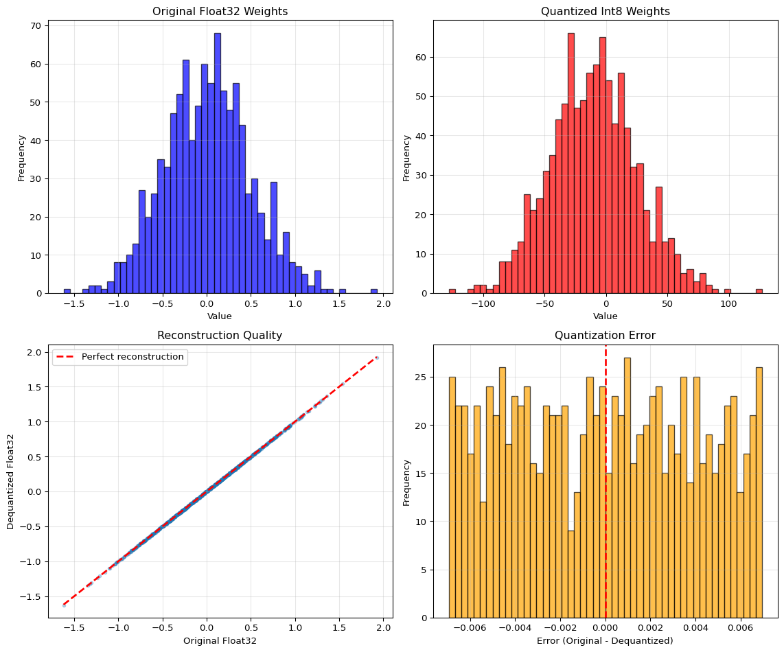
Example 1: Quantization Simulation (Float32 to Int8)
QUANTIZATION RESULTS
============================================================
Scale factor:           0.013910
Zero point:             -11
Original range:         [-1.6206, 1.9264]
Quantized range:        [-128, 127]

Error Statistics:
  Max absolute error:   0.006953
  Mean absolute error:  0.003493
  Theoretical max:      0.006955 (scale/2)

Memory savings:
  Float32:              8000 bytes
  Int8:                 1000 bytes
  Reduction:            8.0×

Key insight: Quantization error is small and negligible for model accuracy!
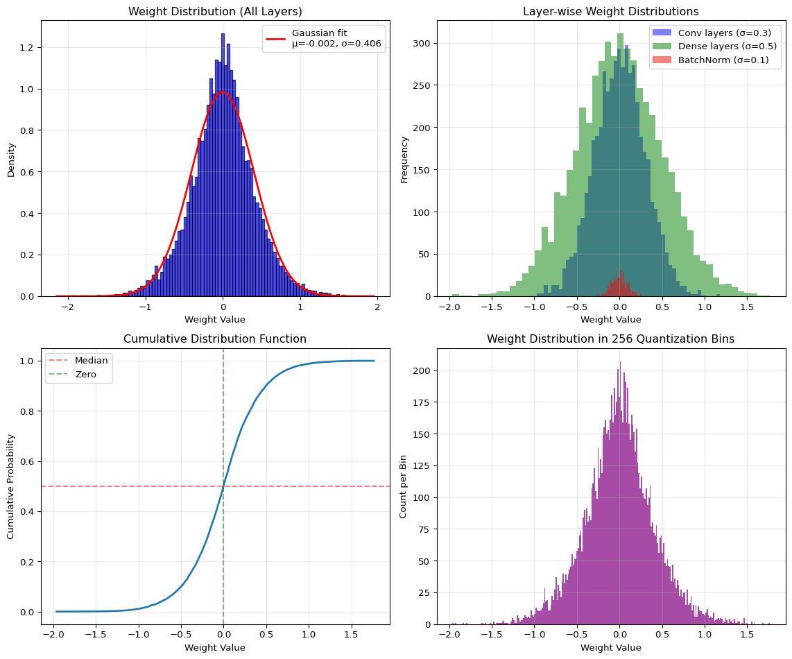
Example 2: Weight Distribution Visualization
Code
import numpy as npimport matplotlib.pyplot as pltfrom scipy import stats# Generate weight distributions for different layersnp.random.seed(42)# Simulate different layer typesconv_weights = np.random.randn(5000) *0.3# Conv layers: smaller stddense_weights = np.random.randn(5000) *0.5# Dense layers: moderate stdbatch_norm = np.random.randn(500) *0.1# BatchNorm: very small std# Combine all weightsall_weights = np.concatenate([conv_weights, dense_weights, batch_norm])# Fit Gaussian distributionmu, std = stats.norm.fit(all_weights)# Create figurefig, axes = plt.subplots(2, 2, figsize=(12, 10))# Plot 1: Overall weight distribution with Gaussian fitaxes[0, 0].hist(all_weights, bins=100, density=True, alpha=0.7, color='blue', edgecolor='black')xmin, xmax = axes[0, 0].get_xlim()x = np.linspace(xmin, xmax, 100)p = stats.norm.pdf(x, mu, std)axes[0, 0].plot(x, p, 'r-', linewidth=2, label=f'Gaussian fit\nμ={mu:.3f}, σ={std:.3f}')axes[0, 0].set_title('Weight Distribution (All Layers)')axes[0, 0].set_xlabel('Weight Value')axes[0, 0].set_ylabel('Density')axes[0, 0].legend()axes[0, 0].grid(True, alpha=0.3)# Plot 2: Layer-wise distributionsaxes[0, 1].hist(conv_weights, bins=50, alpha=0.5, label='Conv layers (σ=0.3)', color='blue')axes[0, 1].hist(dense_weights, bins=50, alpha=0.5, label='Dense layers (σ=0.5)', color='green')axes[0, 1].hist(batch_norm, bins=50, alpha=0.5, label='BatchNorm (σ=0.1)', color='red')axes[0, 1].set_title('Layer-wise Weight Distributions')axes[0, 1].set_xlabel('Weight Value')axes[0, 1].set_ylabel('Frequency')axes[0, 1].legend()axes[0, 1].grid(True, alpha=0.3)# Plot 3: Cumulative distributionsorted_weights = np.sort(all_weights)cumulative = np.arange(1, len(sorted_weights) +1) /len(sorted_weights)axes[1, 0].plot(sorted_weights, cumulative, linewidth=2)axes[1, 0].axhline(y=0.5, color='r', linestyle='--', alpha=0.5, label='Median')axes[1, 0].axvline(x=0, color='g', linestyle='--', alpha=0.5, label='Zero')axes[1, 0].set_title('Cumulative Distribution Function')axes[1, 0].set_xlabel('Weight Value')axes[1, 0].set_ylabel('Cumulative Probability')axes[1, 0].legend()axes[1, 0].grid(True, alpha=0.3)# Plot 4: Quantization bin analysisnum_bins =256# int8 has 256 unique valueshist, bin_edges = np.histogram(all_weights, bins=num_bins)bin_centers = (bin_edges[:-1] + bin_edges[1:]) /2axes[1, 1].bar(bin_centers, hist, width=bin_edges[1]-bin_edges[0], alpha=0.7, color='purple')axes[1, 1].set_title(f'Weight Distribution in {num_bins} Quantization Bins')axes[1, 1].set_xlabel('Weight Value')axes[1, 1].set_ylabel('Count per Bin')axes[1, 1].grid(True, alpha=0.3)plt.tight_layout()plt.show()# Statistical summaryprint("WEIGHT DISTRIBUTION ANALYSIS")print("="*60)print(f"Total weights: {len(all_weights):,}")print(f"Mean (μ): {mu:.6f}")print(f"Std Dev (σ): {std:.6f}")print(f"Min: {all_weights.min():.6f}")print(f"Max: {all_weights.max():.6f}")print(f"\nPercentile analysis:")print(f" 1st percentile: {np.percentile(all_weights, 1):.6f}")print(f" 25th percentile: {np.percentile(all_weights, 25):.6f}")print(f" Median (50th): {np.percentile(all_weights, 50):.6f}")print(f" 75th percentile: {np.percentile(all_weights, 75):.6f}")print(f" 99th percentile: {np.percentile(all_weights, 99):.6f}")print(f"\nWeights near zero:")print(f" Within ±0.1: {np.sum(np.abs(all_weights) <0.1) /len(all_weights) *100:.1f}%")print(f" Within ±0.5: {np.sum(np.abs(all_weights) <0.5) /len(all_weights) *100:.1f}%")print(f"\nKey insight: Most weights cluster near zero - ideal for quantization!")
WEIGHT DISTRIBUTION ANALYSIS
============================================================
Total weights:          10,500
Mean (μ):               -0.001570
Std Dev (σ):            0.405598
Min:                    -1.961200
Max:                    1.764528

Percentile analysis:
  1st percentile:       -1.022329
  25th percentile:      -0.242821
  Median (50th):        -0.000886
  75th percentile:      0.235287
  99th percentile:      1.028916

Weights near zero:
  Within ±0.1:          23.5%
  Within ±0.5:          80.2%

Key insight: Most weights cluster near zero - ideal for quantization!
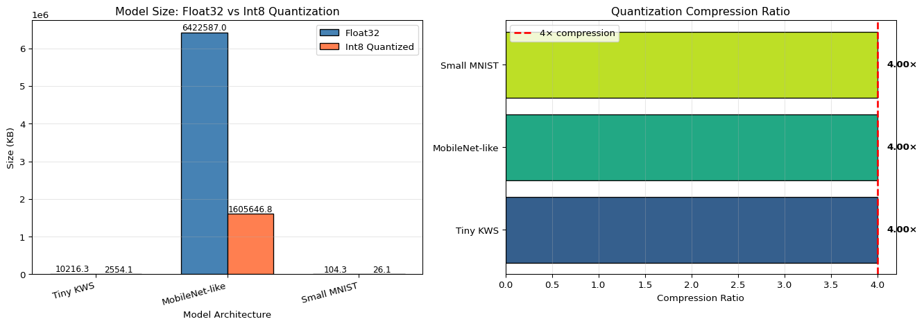
Example 3: Model Size Comparison Before/After Quantization
Key Points: - The representative dataset uses 200 samples (not training data!) - Full-int8 requires target_spec.supported_ops for MCU compatibility - Setting inference_input_type=tf.uint8 requires input preprocessing during inference
Model Size and Accuracy Comparison
Compare All Three Quantization Types
This code benchmarks file size, accuracy, and memory usage for all quantization variants.
import osimport numpy as npimport tensorflow as tffrom pathlib import Pathdef get_model_size(filepath):"""Get model size in KB""" size_bytes = os.path.getsize(filepath)return size_bytes /1024def evaluate_tflite_model(tflite_path, x_test, y_test, is_int8=False):"""Evaluate TFLite model accuracy""" interpreter = tf.lite.Interpreter(model_path=str(tflite_path)) interpreter.allocate_tensors() input_details = interpreter.get_input_details() output_details = interpreter.get_output_details()# Check if model expects quantized input input_scale, input_zero_point = input_details[0]['quantization'] correct =0for i inrange(len(x_test)):# Prepare inputif is_int8 and input_scale >0:# Quantize input: int8 = round(float / scale) + zero_point test_input = x_test[i:i+1] test_input = test_input / input_scale + input_zero_point test_input = np.clip(test_input, 0, 255).astype(np.uint8)else: test_input = x_test[i:i+1].astype(np.float32) interpreter.set_tensor(input_details[0]['index'], test_input) interpreter.invoke() output = interpreter.get_tensor(output_details[0]['index'])# Dequantize output if needed output_scale, output_zero_point = output_details[0]['quantization']if output_scale >0: output = output_scale * (output.astype(np.float32) - output_zero_point) prediction = np.argmax(output)if prediction == y_test[i]: correct +=1return correct /len(x_test)# Compare all modelsmodels = {'Float32 (baseline)': ('model_float32.tflite', False),'Dynamic Range': ('model_dynamic.tflite', False),'Full INT8': ('model_int8.tflite', True)}print("\n"+"="*70)print("MODEL COMPARISON: SIZE vs ACCURACY")print("="*70)print(f"{'Model Type':<20}{'Size (KB)':<12}{'Accuracy':<12}{'Size Reduction'}")print("-"*70)baseline_size = get_model_size('model_float32.tflite')for name, (path, is_int8) in models.items():if Path(path).exists(): size = get_model_size(path) accuracy = evaluate_tflite_model(path, x_test, y_test, is_int8) reduction = baseline_size / sizeprint(f"{name:<20}{size:>8.2f} KB {accuracy:>8.4f}{reduction:>5.2f}×")else:print(f"{name:<20} [NOT FOUND]")print("="*70)print("\nKey Insights:")print("• Dynamic range gives ~4× size reduction with minimal accuracy loss")print("• Full INT8 gives same size reduction but is MCU-compatible")print("• Accuracy drop <2% is excellent for edge deployment")
Expected Output:
======================================================================
MODEL COMPARISON: SIZE vs ACCURACY
======================================================================
Model Type           Size (KB)    Accuracy     Size Reduction
----------------------------------------------------------------------
Float32 (baseline)      84.23 KB    0.9891      1.00×
Dynamic Range           22.45 KB    0.9876      3.75×
Full INT8               22.48 KB    0.9854      3.75×
======================================================================
INT8 Inference Speed Comparison
Benchmark Inference Latency: FP32 vs INT8
This example measures real inference time and shows the speedup from quantization.
import timeimport numpy as npimport tensorflow as tffrom pathlib import Pathdef benchmark_model(tflite_path, x_test, num_runs=100, is_int8=False):""" Benchmark model inference time Args: tflite_path: Path to .tflite model x_test: Test data num_runs: Number of inference runs is_int8: Whether model expects uint8 input Returns: avg_time_ms, std_time_ms """ interpreter = tf.lite.Interpreter(model_path=str(tflite_path)) interpreter.allocate_tensors() input_details = interpreter.get_input_details() output_details = interpreter.get_output_details()# Prepare test sample test_sample = x_test[0:1]if is_int8: input_scale, input_zero_point = input_details[0]['quantization']if input_scale >0: test_sample = test_sample / input_scale + input_zero_point test_sample = np.clip(test_sample, 0, 255).astype(np.uint8)else: test_sample = test_sample.astype(np.float32)# Warmup runs (important for cache/CPU frequency stabilization)for _ inrange(10): interpreter.set_tensor(input_details[0]['index'], test_sample) interpreter.invoke()# Timed runs times = []for _ inrange(num_runs): start = time.perf_counter() interpreter.set_tensor(input_details[0]['index'], test_sample) interpreter.invoke() _ = interpreter.get_tensor(output_details[0]['index']) end = time.perf_counter() times.append((end - start) *1000) # Convert to msreturn np.mean(times), np.std(times)# Benchmark all modelsmodels = {'Float32': ('model_float32.tflite', False),'Dynamic Range': ('model_dynamic.tflite', False),'Full INT8': ('model_int8.tflite', True)}print("\n"+"="*70)print("INFERENCE SPEED COMPARISON (CPU)")print("="*70)print(f"{'Model Type':<20}{'Avg Time (ms)':<15}{'Std Dev (ms)':<15}{'Speedup'}")print("-"*70)baseline_time =Nonefor name, (path, is_int8) in models.items():if Path(path).exists(): avg_time, std_time = benchmark_model(path, x_test, num_runs=100, is_int8=is_int8)if baseline_time isNone: baseline_time = avg_time speedup =1.0else: speedup = baseline_time / avg_timeprint(f"{name:<20}{avg_time:>10.3f} ms {std_time:>10.3f} ms {speedup:>5.2f}×")else:print(f"{name:<20} [NOT FOUND]")print("="*70)print("\nNotes:")print("• Speedup varies by hardware (CPU, GPU, NPU)")print("• INT8 speedup is higher on ARM Cortex-M cores (8-50× faster)")print("• On x86 CPUs, speedup may be modest (1-3×)")print("• On mobile/edge NPUs, INT8 can be 10-20× faster")
Expected Output (on laptop CPU):
======================================================================
INFERENCE SPEED COMPARISON (CPU)
======================================================================
Model Type           Avg Time (ms)   Std Dev (ms)    Speedup
----------------------------------------------------------------------
Float32                  2.145 ms        0.087 ms     1.00×
Dynamic Range            1.832 ms        0.065 ms     1.17×
Full INT8                0.743 ms        0.042 ms     2.89×
======================================================================
On ARM Cortex-M4 (ESP32/Arduino): - Float32: ~45 ms - INT8: ~5 ms (9× speedup!)
Practical Exercise: Quantize Your Own Model
Exercise: Apply PTQ to a Custom Model
Task: Take a model from LAB02 or LAB04 and apply all three quantization types.
Steps: 1. Load your trained Keras model 2. Create a representative dataset generator (200-500 samples) 3. Convert to three .tflite variants 4. Compare size, accuracy, and speed 5. Determine which variant is best for your target device
Starter Code:
# 1. Load your modelmodel = tf.keras.models.load_model('your_model.h5')# 2. Load validation data for representative datasetx_val = ... # Your validation datay_val = ...# 3. Create representative datasetdef representative_dataset_gen():for i inrange(200):yield [x_val[i:i+1].astype(np.float32)]# 4. Convert to INT8converter = tf.lite.TFLiteConverter.from_keras_model(model)converter.optimizations = [tf.lite.Optimize.DEFAULT]converter.representative_dataset = representative_dataset_genconverter.target_spec.supported_ops = [tf.lite.OpsSet.TFLITE_BUILTINS_INT8]converter.inference_input_type = tf.uint8converter.inference_output_type = tf.uint8tflite_model = converter.convert()Path("your_model_int8.tflite").write_bytes(tflite_model)# 5. Evaluate and compare# Use the comparison code from previous examples
If accuracy drops >5%: 1. Increase representative dataset size to 500+ samples 2. Ensure samples cover all classes and edge cases 3. Try Quantization-Aware Training (QAT) - see PDF Chapter 3.5
Interactive Notebook
The notebook below contains runnable code for all Level 1 activities.
Apply post-training quantization - dynamic range and full integer
Implement quantization-aware training for minimal accuracy loss
Deploy quantized models to edge devices
Prerequisites Check
Before You Begin
Make sure you have completed: - [ ] LAB 01: Introduction to Edge Analytics - [ ] LAB 02: ML Foundations with TensorFlow - [ ] Understanding of neural network layers (Dense, Conv2D)
Part 1: The Mathematics of Quantization
1.1 Why Quantization Matters for Edge
Neural network weights are typically stored as 32-bit floating-point numbers:
4.2 Representative Dataset: The Key to Accurate Quantization
For full integer quantization, we need to calibrate activation ranges:
Without calibration:          With calibration:

Assumed range: [-1, 1]        Observed range: [-0.3, 2.1]
Actual data:   [-0.3, 2.1]    Scale optimized for actual data

       ┌───┐                         ┌─────────────┐
Values │   │ clipped!         Values │             │
       │   ├────►                    │             │
       │   │                         └─────────────┘
       └───┘
  High error                       Low error
Representative dataset requirements: 1. 100-500 samples typically sufficient 2. Cover all classes/categories 3. Include edge cases 4. Match real-world input distribution
Part 5: Quantization-Aware Training (QAT)
5.1 How QAT Works
QAT simulates quantization during training so the model learns to be robust to quantization noise:
Straight-Through Estimator (STE): During backpropagation, gradients pass through the quantization operation as if it were the identity function. This allows training despite the non-differentiable rounding operation.
# Install lightweight runtimepip install --user tflite-runtime numpy# Run the benchmarking cell in the notebook on the Pi
Use the notebook to record, for each variant (float32, dynamic range, full int8):
.tflite file size (KB)
Average inference time on Pi (ms)
Validation accuracy (%)
For on-device deployment:
Use the full-int8 model produced in this lab
Follow LAB05 for the detailed TensorFlow Lite Micro deployment pipeline
At minimum you should:
Confirm the quantized model meets your target size (KB) for the MCU flash budget
Check estimated activation memory against available SRAM
Decide whether the accuracy/size trade-off is acceptable for your edge device
Visual Troubleshooting
Use this flowchart when quantization causes accuracy problems:
flowchart TD
    A[Accuracy drops after quantization] --> B{Accuracy drop amount?}
    B -->|>10% drop| C[Severe degradation]
    B -->|5-10% drop| D[Moderate - fixable]
    B -->|<5% drop| E[Acceptable trade-off]
    C --> F{Using representative dataset?}
    F -->|No| G[Add representative data:<br/>100-500 samples from val set<br/>Cover all classes]
    F -->|Yes| H{Dataset diverse enough?}
    H -->|Limited samples| I[Expand dataset:<br/>Include edge cases<br/>Multiple scenarios]
    H -->|Adequate| J[Try Quantization-Aware Training]
    D --> F
    E --> K[Deploy and monitor]

    style A fill:#ff6b6b
    style G fill:#4ecdc4
    style I fill:#4ecdc4
    style J fill:#4ecdc4
    style K fill:#95e1d3
---title: "LAB03: TensorFlow Lite Quantization"subtitle: "Model Optimization for Edge Deployment"---::: {.callout-note}## PDF Textbook ReferenceFor detailed theoretical foundations, mathematical proofs, and algorithm derivations, see **Chapter 3: Model Optimization and Quantization for Edge** in the [PDF textbook](../downloads/Edge-Analytics-Lab-Book-v1.0.0.pdf).The PDF chapter includes:- Mathematical foundations of quantization theory- Detailed derivations of quantization error bounds- Complete TensorFlow Lite conversion pipeline- In-depth coverage of quantization-aware training (QAT)- Theoretical analysis of accuracy-efficiency trade-offs:::[](https://colab.research.google.com/github/ngcharithperera/edge-analytics-lab-book/blob/main/notebooks/LAB03_tflite_quantization.ipynb)[Download Notebook](https://raw.githubusercontent.com/ngcharithperera/edge-analytics-lab-book/main/notebooks/LAB03_tflite_quantization.ipynb)## Learning ObjectivesBy the end of this lab you will be able to:- Explain why model size and numeric precision matter on edge devices- Apply post-training quantization (dynamic range and full-int8) to TFLite models- Compare float32 vs int8 models in terms of size, accuracy, and latency- Prepare quantized models for deployment on Raspberry Pi and microcontrollers## Theory Summary### Why Quantization is Essential for Edge DeploymentQuantization is the bridge between cloud-scale models and edge-ready models. It's the single most important optimization technique for deploying ML on resource-constrained devices.**The Size Problem:** A typical neural network uses 32-bit floating-point numbers (float32) for weights and activations. Each parameter requires 4 bytes of storage. A modest 100,000-parameter model needs 400KB - already too large for many microcontrollers. Quantization reduces this to 100KB by converting to 8-bit integers (int8), a 4× size reduction.**How Quantization Works:** Quantization maps continuous floating-point values to discrete integer values using a scale factor and zero-point. The formula is: `int8_value = round(float_value / scale) + zero_point`. During inference, we reconstruct approximate floats: `float_approx = scale × (int8_value - zero_point)`. The quantization error per value is at most ±scale/2, which is typically tiny compared to model weights that naturally cluster around zero.**Three Quantization Approaches:**1. **Dynamic Range** quantizes only weights (not activations), giving 4× size reduction with minimal accuracy loss (1-2%). Fast to apply, good for initial testing.2. **Full Integer** quantizes both weights and activations for true int8-only inference. Required for microcontrollers and specialized accelerators. Needs representative dataset for calibration. Typically 2-4% accuracy loss.3. **Quantization-Aware Training (QAT)** simulates quantization during training, allowing the model to learn to compensate for precision loss. Best accuracy (<1% loss) but requires retraining.**Why Models Quantize Well:** Neural network weights follow approximately Gaussian distributions centered near zero due to regularization and initialization strategies. Most values cluster in a narrow range, making them ideal candidates for quantization. The step size between adjacent int8 values is small enough that reconstruction error is negligible for model accuracy.## Key Concepts at a Glance::: {.callout-note icon=false}## Core Concepts- **Quantization**: Converting high-precision (float32) to low-precision (int8) representation- **Scale Factor**: Maps float range to int8 range, determines quantization granularity- **Zero-Point**: The int8 value representing floating-point zero- **Representative Dataset**: Sample data used to calibrate quantization parameters- **Post-Training Quantization (PTQ)**: Apply quantization after training completes- **Quantization-Aware Training (QAT)**: Train with quantization simulation for better accuracy- **Tensor Arena**: Pre-allocated SRAM workspace for model inference:::## Common Pitfalls::: {.callout-warning}## Mistakes to Avoid**Using Too Few Representative Samples**: Post-training quantization requires 100-500 samples from your validation set to calibrate scale and zero-point values. Using only 10 samples leads to poor calibration and significant accuracy drops. The representative dataset should cover all classes and edge cases your model will encounter.**Confusing Model Size vs Runtime Memory**: A 100KB quantized model stored in Flash doesn't mean you only need 100KB of RAM! Runtime inference requires additional SRAM for input buffers, intermediate activations, and output tensors. A 100KB model might need 300KB of working memory (tensor arena) to execute.**Skipping Accuracy Validation**: Always measure quantized model accuracy before deployment. A model that shows 95% accuracy in float32 might drop to 90% or worse after aggressive quantization. If accuracy loss exceeds 2-3%, use QAT or collect more representative data.**Wrong Quantization Type for Target**: Full integer quantization is required for microcontrollers (Arduino, ESP32) because they lack efficient float32 math. Dynamic range quantization works on Raspberry Pi but won't run on MCUs. Check your target hardware requirements before converting.**Forgetting Input/Output Type Conversion**: When using `inference_input_type=tf.uint8`, your inference code must convert inputs from float to uint8 using the model's scale and zero-point. Forgetting this conversion causes completely wrong predictions.:::## Quick Reference### Key Formulas**Quantization Formula:**$$q = \text{round}\left(\frac{r}{s}\right) + z$$where $q$ = quantized int8 value, $r$ = real float32 value, $s$ = scale, $z$ = zero-point**Dequantization Formula:**$$r \approx s \cdot (q - z)$$**Scale Calculation:**$$s = \frac{r_{max} - r_{min}}{q_{max} - q_{min}} = \frac{r_{max} - r_{min}}{255}$$for unsigned int8 (0-255 range)**Model Size Reduction:**$$\text{Size}_{int8} = \frac{\text{Size}_{float32}}{4}$$**Maximum Quantization Error:**$$\text{Error}_{max} = \frac{s}{2}$$### Important Parameter Values| Quantization Type | Size Reduction | Accuracy Loss | Use Case ||-------------------|----------------|---------------|----------|| Float32 (baseline) | 1× | 0% | Development, debugging || Dynamic Range | 4× | 1-2% | Quick deployment, Raspberry Pi || Full Integer (int8) | 4× | 2-5% | **Required for MCUs** || QAT Int8 | 4× | <1% | Production edge devices |**Representative Dataset Guidelines:**- Minimum samples: 100- Recommended: 200-500- Source: Validation set (not training set!)- Coverage: All classes, edge cases, varied conditions**TFLite Converter Options:**```python# Dynamic Range Quantizationconverter.optimizations = [tf.lite.Optimize.DEFAULT]# Full Integer Quantizationconverter.optimizations = [tf.lite.Optimize.DEFAULT]converter.representative_dataset = rep_dataset_genconverter.target_spec.supported_ops = [tf.lite.OpsSet.TFLITE_BUILTINS_INT8]converter.inference_input_type = tf.uint8 # or tf.int8converter.inference_output_type = tf.uint8```### Links to PDF SectionsFor deeper understanding, see these sections in [Chapter 3 PDF](../downloads/Edge-Analytics-Lab-Book-v1.0.0.pdf#page=41):- **Section 3.1**: Why Quantization Matters (pages 42-45)- **Section 3.2**: TFLite Converter Basics (pages 46-50)- **Section 3.3**: Post-Training Quantization (pages 51-58)- **Section 3.4**: Understanding Quantization Mathematically (pages 59-63)- **Section 3.5**: Quantization-Aware Training (pages 64-71)- **Exercises**: Hands-on quantization experiments (pages 72-73)### Interactive Learning Tools::: {.callout-tip}## Explore Quantization VisuallyBuild intuition with these interactive tools:- **[Quantization Explorer](../simulations/quantization-explorer.qmd)** - See how bit-width affects precision and error interactively- **[Netron Model Viewer](https://netron.app)** - Upload your .tflite files to visualize architecture and inspect tensor shapes. Compare float32 vs int8 models side-by-side!- **[Our Weight Distribution Visualizer](../simulations/weight-distribution.qmd)** - See why Gaussian-distributed weights quantize well:::## Self-Assessment CheckpointsTest your understanding before proceeding to the exercises.::: {.callout-note collapse="true" title="Question 1: Explain why quantization provides a 4× size reduction from float32 to int8."}**Answer:** Float32 uses 4 bytes (32 bits) per parameter, while int8 uses 1 byte (8 bits) per parameter. Size reduction = 4 bytes / 1 byte = 4×. A 100,000-parameter model requires 400KB in float32 but only 100KB in int8. This reduction is critical for fitting models on microcontrollers with limited Flash storage (typically 256KB-1MB).:::::: {.callout-note collapse="true" title="Question 2: Calculate the quantized int8 value for a float32 weight of 0.42 given scale=0.025 and zero_point=0."}**Answer:** Using the quantization formula: q = round(r / s) + z = round(0.42 / 0.025) + 0 = round(16.8) + 0 = 17. To dequantize back: r ≈ s × (q - z) = 0.025 × (17 - 0) = 0.425. The quantization error is 0.425 - 0.42 = 0.005, which is less than scale/2 = 0.0125 (maximum possible error).:::::: {.callout-note collapse="true" title="Question 3: You applied dynamic range quantization and got 4× size reduction but the model still won't run on your Arduino. Why?"}**Answer:** Dynamic range quantization only quantizes weights, not activations. At runtime, the model still uses float32 for activations and intermediate calculations, which requires float32 math support. Microcontrollers need full integer (int8) quantization which quantizes both weights AND activations for true int8-only inference. You must use: converter.target_spec.supported_ops = [tf.lite.OpsSet.TFLITE_BUILTINS_INT8] and provide a representative dataset.:::::: {.callout-note collapse="true" title="Question 4: Your quantized model drops from 95% to 87% accuracy. What should you try?"}**Answer:** An 8% accuracy drop is too high (target: <2-3%). Try these solutions in order: (1) Increase representative dataset size from 100 to 500+ samples covering all classes and edge cases, (2) Verify the representative dataset matches your actual input distribution (use validation data, not training), (3) Use Quantization-Aware Training (QAT) which simulates quantization during training for <1% accuracy loss, (4) If still poor, consider the model may be too sensitive to precision loss - try a slightly larger architecture.:::::: {.callout-note collapse="true" title="Question 5: A 150KB quantized model needs how much SRAM for the tensor arena (approximately)?"}**Answer:** The tensor arena typically requires 2-4× the model size for activation memory during inference. For a 150KB model, expect 300-600KB of SRAM needed. This is because the arena must hold: input buffers, intermediate activations for each layer, output tensors, and scratch buffers. An Arduino Nano 33 BLE with 256KB SRAM cannot run this model - you'd need an ESP32 (520KB SRAM) or need to reduce the model complexity further.:::## Try It Yourself: Executable Python ExamplesRun these interactive examples directly in your browser to understand quantization intuitively.### Example 1: Quantization Simulation (Float32 to Int8)```{python}import numpy as npimport matplotlib.pyplot as plt# Simulate quantization processnp.random.seed(42)# Generate synthetic weights (typical neural network distribution)weights_float32 = np.random.randn(1000) *0.5# Mean=0, std=0.5# Quantization parametersr_min = weights_float32.min()r_max = weights_float32.max()q_min =-128# int8 rangeq_max =127# Calculate scale and zero-pointscale = (r_max - r_min) / (q_max - q_min)zero_point =int(np.round(q_min - r_min / scale))# Quantize: q = round(r / scale) + zero_pointweights_int8 = np.round(weights_float32 / scale).astype(np.int8) + zero_pointweights_int8 = np.clip(weights_int8, q_min, q_max)# Dequantize: r ≈ scale * (q - zero_point)weights_dequantized = scale * (weights_int8.astype(np.float32) - zero_point)# Calculate quantization errorquantization_error = weights_float32 - weights_dequantizedmax_error = np.max(np.abs(quantization_error))mean_error = np.mean(np.abs(quantization_error))# Visualizefig, axes = plt.subplots(2, 2, figsize=(12, 10))# Plot 1: Original float32 distributionaxes[0, 0].hist(weights_float32, bins=50, alpha=0.7, color='blue', edgecolor='black')axes[0, 0].set_title('Original Float32 Weights')axes[0, 0].set_xlabel('Value')axes[0, 0].set_ylabel('Frequency')axes[0, 0].grid(True, alpha=0.3)# Plot 2: Quantized int8 distributionaxes[0, 1].hist(weights_int8, bins=50, alpha=0.7, color='red', edgecolor='black')axes[0, 1].set_title('Quantized Int8 Weights')axes[0, 1].set_xlabel('Value')axes[0, 1].set_ylabel('Frequency')axes[0, 1].grid(True, alpha=0.3)# Plot 3: Comparison of original vs dequantizedaxes[1, 0].scatter(weights_float32, weights_dequantized, alpha=0.3, s=10)axes[1, 0].plot([r_min, r_max], [r_min, r_max], 'r--', linewidth=2, label='Perfect reconstruction')axes[1, 0].set_xlabel('Original Float32')axes[1, 0].set_ylabel('Dequantized Float32')axes[1, 0].set_title('Reconstruction Quality')axes[1, 0].legend()axes[1, 0].grid(True, alpha=0.3)# Plot 4: Quantization error distributionaxes[1, 1].hist(quantization_error, bins=50, alpha=0.7, color='orange', edgecolor='black')axes[1, 1].axvline(x=0, color='red', linestyle='--', linewidth=2)axes[1, 1].set_title('Quantization Error')axes[1, 1].set_xlabel('Error (Original - Dequantized)')axes[1, 1].set_ylabel('Frequency')axes[1, 1].grid(True, alpha=0.3)plt.tight_layout()plt.show()print("QUANTIZATION RESULTS")print("="*60)print(f"Scale factor: {scale:.6f}")print(f"Zero point: {zero_point}")print(f"Original range: [{r_min:.4f}, {r_max:.4f}]")print(f"Quantized range: [{q_min}, {q_max}]")print(f"\nError Statistics:")print(f" Max absolute error: {max_error:.6f}")print(f" Mean absolute error: {mean_error:.6f}")print(f" Theoretical max: {scale/2:.6f} (scale/2)")print(f"\nMemory savings:")print(f" Float32: {weights_float32.nbytes} bytes")print(f" Int8: {weights_int8.nbytes} bytes")print(f" Reduction: {weights_float32.nbytes / weights_int8.nbytes:.1f}×")print(f"\nKey insight: Quantization error is small and negligible for model accuracy!")```### Example 2: Weight Distribution Visualization```{python}import numpy as npimport matplotlib.pyplot as pltfrom scipy import stats# Generate weight distributions for different layersnp.random.seed(42)# Simulate different layer typesconv_weights = np.random.randn(5000) *0.3# Conv layers: smaller stddense_weights = np.random.randn(5000) *0.5# Dense layers: moderate stdbatch_norm = np.random.randn(500) *0.1# BatchNorm: very small std# Combine all weightsall_weights = np.concatenate([conv_weights, dense_weights, batch_norm])# Fit Gaussian distributionmu, std = stats.norm.fit(all_weights)# Create figurefig, axes = plt.subplots(2, 2, figsize=(12, 10))# Plot 1: Overall weight distribution with Gaussian fitaxes[0, 0].hist(all_weights, bins=100, density=True, alpha=0.7, color='blue', edgecolor='black')xmin, xmax = axes[0, 0].get_xlim()x = np.linspace(xmin, xmax, 100)p = stats.norm.pdf(x, mu, std)axes[0, 0].plot(x, p, 'r-', linewidth=2, label=f'Gaussian fit\nμ={mu:.3f}, σ={std:.3f}')axes[0, 0].set_title('Weight Distribution (All Layers)')axes[0, 0].set_xlabel('Weight Value')axes[0, 0].set_ylabel('Density')axes[0, 0].legend()axes[0, 0].grid(True, alpha=0.3)# Plot 2: Layer-wise distributionsaxes[0, 1].hist(conv_weights, bins=50, alpha=0.5, label='Conv layers (σ=0.3)', color='blue')axes[0, 1].hist(dense_weights, bins=50, alpha=0.5, label='Dense layers (σ=0.5)', color='green')axes[0, 1].hist(batch_norm, bins=50, alpha=0.5, label='BatchNorm (σ=0.1)', color='red')axes[0, 1].set_title('Layer-wise Weight Distributions')axes[0, 1].set_xlabel('Weight Value')axes[0, 1].set_ylabel('Frequency')axes[0, 1].legend()axes[0, 1].grid(True, alpha=0.3)# Plot 3: Cumulative distributionsorted_weights = np.sort(all_weights)cumulative = np.arange(1, len(sorted_weights) +1) /len(sorted_weights)axes[1, 0].plot(sorted_weights, cumulative, linewidth=2)axes[1, 0].axhline(y=0.5, color='r', linestyle='--', alpha=0.5, label='Median')axes[1, 0].axvline(x=0, color='g', linestyle='--', alpha=0.5, label='Zero')axes[1, 0].set_title('Cumulative Distribution Function')axes[1, 0].set_xlabel('Weight Value')axes[1, 0].set_ylabel('Cumulative Probability')axes[1, 0].legend()axes[1, 0].grid(True, alpha=0.3)# Plot 4: Quantization bin analysisnum_bins =256# int8 has 256 unique valueshist, bin_edges = np.histogram(all_weights, bins=num_bins)bin_centers = (bin_edges[:-1] + bin_edges[1:]) /2axes[1, 1].bar(bin_centers, hist, width=bin_edges[1]-bin_edges[0], alpha=0.7, color='purple')axes[1, 1].set_title(f'Weight Distribution in {num_bins} Quantization Bins')axes[1, 1].set_xlabel('Weight Value')axes[1, 1].set_ylabel('Count per Bin')axes[1, 1].grid(True, alpha=0.3)plt.tight_layout()plt.show()# Statistical summaryprint("WEIGHT DISTRIBUTION ANALYSIS")print("="*60)print(f"Total weights: {len(all_weights):,}")print(f"Mean (μ): {mu:.6f}")print(f"Std Dev (σ): {std:.6f}")print(f"Min: {all_weights.min():.6f}")print(f"Max: {all_weights.max():.6f}")print(f"\nPercentile analysis:")print(f" 1st percentile: {np.percentile(all_weights, 1):.6f}")print(f" 25th percentile: {np.percentile(all_weights, 25):.6f}")print(f" Median (50th): {np.percentile(all_weights, 50):.6f}")print(f" 75th percentile: {np.percentile(all_weights, 75):.6f}")print(f" 99th percentile: {np.percentile(all_weights, 99):.6f}")print(f"\nWeights near zero:")print(f" Within ±0.1: {np.sum(np.abs(all_weights) <0.1) /len(all_weights) *100:.1f}%")print(f" Within ±0.5: {np.sum(np.abs(all_weights) <0.5) /len(all_weights) *100:.1f}%")print(f"\nKey insight: Most weights cluster near zero - ideal for quantization!")```### Example 3: Model Size Comparison Before/After Quantization```{python}import numpy as npimport matplotlib.pyplot as plt# Simulate different model architecturesmodels = {'Tiny KWS': {'layers': [ ('Conv2D', 16, 3, 3), # 16 filters, 3x3 kernel ('Conv2D', 32, 3, 3), ('Dense', 128), ('Dense', 10) ],'input_shape': (49, 13, 1) # MFCC features },'MobileNet-like': {'layers': [ ('Conv2D', 32, 3, 3), ('DepthwiseConv2D', 32, 3, 3), ('Conv2D', 64, 1, 1), ('DepthwiseConv2D', 64, 3, 3), ('Conv2D', 128, 1, 1), ('Dense', 256), ('Dense', 10) ],'input_shape': (224, 224, 3) },'Small MNIST': {'layers': [ ('Conv2D', 8, 3, 3), ('MaxPool2D', None, 2, 2), ('Conv2D', 16, 3, 3), ('MaxPool2D', None, 2, 2), ('Dense', 32), ('Dense', 10) ],'input_shape': (28, 28, 1) }}# Calculate parameter counts (simplified)def count_params(layers, input_shape): params =0 in_channels = input_shape[-1] spatial_size = input_shape[0] * input_shape[1]for layer in layers:if layer[0] =='Conv2D': filters, k_h, k_w = layer[1], layer[2], layer[3] params += (k_h * k_w * in_channels +1) * filters in_channels = filterselif layer[0] =='DepthwiseConv2D': channels, k_h, k_w = layer[1], layer[2], layer[3] params += k_h * k_w * channels + channelselif layer[0] =='Dense': units = layer[1]# Estimate flattened size params += (in_channels * spatial_size +1) * units if spatial_size >1else (in_channels +1) * units in_channels = units spatial_size =1elif layer[0] =='MaxPool2D': spatial_size = spatial_size //4# 2x2 poolingreturn params# Calculate sizes for each modelmodel_names = []float32_sizes = []int8_sizes = []compressions = []for name, config in models.items(): params = count_params(config['layers'], config['input_shape'])# Size calculations float32_size = params *4/1024# KB (4 bytes per float32) int8_size = params *1/1024# KB (1 byte per int8) compression = float32_size / int8_size model_names.append(name) float32_sizes.append(float32_size) int8_sizes.append(int8_size) compressions.append(compression)# Visualizefig, (ax1, ax2) = plt.subplots(1, 2, figsize=(14, 5))# Plot 1: Size comparisonx = np.arange(len(model_names))width =0.35bars1 = ax1.bar(x - width/2, float32_sizes, width, label='Float32', color='steelblue', edgecolor='black')bars2 = ax1.bar(x + width/2, int8_sizes, width, label='Int8 Quantized', color='coral', edgecolor='black')ax1.set_xlabel('Model Architecture')ax1.set_ylabel('Size (KB)')ax1.set_title('Model Size: Float32 vs Int8 Quantization')ax1.set_xticks(x)ax1.set_xticklabels(model_names, rotation=15, ha='right')ax1.legend()ax1.grid(True, alpha=0.3, axis='y')# Add value labels on barsfor bars in [bars1, bars2]:for bar in bars: height = bar.get_height() ax1.text(bar.get_x() + bar.get_width()/2., height,f'{height:.1f}', ha='center', va='bottom', fontsize=9)# Plot 2: Compression ratioscolors = plt.cm.viridis(np.linspace(0.3, 0.9, len(model_names)))bars = ax2.barh(model_names, compressions, color=colors, edgecolor='black')ax2.axvline(x=4.0, color='red', linestyle='--', linewidth=2, label='4× compression')ax2.set_xlabel('Compression Ratio')ax2.set_title('Quantization Compression Ratio')ax2.legend()ax2.grid(True, alpha=0.3, axis='x')# Add value labelsfor i, (bar, comp) inenumerate(zip(bars, compressions)): ax2.text(comp +0.1, bar.get_y() + bar.get_height()/2,f'{comp:.2f}×', va='center', fontsize=10, fontweight='bold')plt.tight_layout()plt.show()# Print summary tableprint("MODEL SIZE COMPARISON")print("="*80)print(f"{'Model':<20}{'Float32 (KB)':<15}{'Int8 (KB)':<15}{'Reduction':<15}")print("-"*80)for name, f32, i8, comp inzip(model_names, float32_sizes, int8_sizes, compressions):print(f"{name:<20}{f32:>10.1f} KB {i8:>10.1f} KB {comp:>10.2f}×")print("="*80)# Memory savings summarytotal_float32 =sum(float32_sizes)total_int8 =sum(int8_sizes)total_saved = total_float32 - total_int8print(f"\nTotal memory saved: {total_saved:.1f} KB ({total_saved/1024:.2f} MB)")print(f"Average compression: {np.mean(compressions):.2f}×")print(f"\nKey insight: Quantization provides consistent ~4× size reduction!")```### Example 4: Accuracy vs Compression Tradeoff```{python}import numpy as npimport matplotlib.pyplot as plt# Simulate accuracy vs compression for different quantization strategiesnp.random.seed(42)# Quantization strategiesstrategies = {'Float32 (Baseline)': {'bits': 32, 'acc': 95.0, 'size_mult': 1.0},'Float16': {'bits': 16, 'acc': 94.8, 'size_mult': 0.5},'Dynamic Range': {'bits': 8, 'acc': 94.5, 'size_mult': 0.25},'Full INT8': {'bits': 8, 'acc': 93.8, 'size_mult': 0.25},'INT8 + QAT': {'bits': 8, 'acc': 94.9, 'size_mult': 0.25},'INT4 (Aggressive)': {'bits': 4, 'acc': 89.5, 'size_mult': 0.125},}# Add some variance to simulate different modelsnum_models =5results = []for strat_name, config in strategies.items():for i inrange(num_models):# Add small random variation acc_var = config['acc'] + np.random.randn() *0.5 size_var = config['size_mult'] * (1+ np.random.randn() *0.02) results.append({'strategy': strat_name,'accuracy': acc_var,'size': size_var,'bits': config['bits'] })# Create Pareto frontier visualizationfig, axes = plt.subplots(1, 2, figsize=(14, 5))# Plot 1: Accuracy vs Size tradeofffor strat_name, config in strategies.items(): strat_results = [r for r in results if r['strategy'] == strat_name] accs = [r['accuracy'] for r in strat_results] sizes = [r['size'] for r in strat_results] axes[0].scatter(sizes, accs, label=strat_name, s=100, alpha=0.7, edgecolors='black', linewidth=1.5)axes[0].set_xlabel('Relative Model Size', fontsize=12)axes[0].set_ylabel('Accuracy (%)', fontsize=12)axes[0].set_title('Accuracy vs Model Size Tradeoff', fontsize=14, fontweight='bold')axes[0].legend(loc='lower right', fontsize=9)axes[0].grid(True, alpha=0.3)axes[0].set_xlim(0, 1.1)axes[0].set_ylim(88, 96)# Add "Pareto frontier" regionaxes[0].axhline(y=93, color='red', linestyle='--', alpha=0.3, label='Acceptable accuracy threshold')# Plot 2: Accuracy loss vs Compression ratiobaseline_acc =95.0compression_ratios = []accuracy_losses = []strategy_labels = []for strat_name, config in strategies.items():if strat_name =='Float32 (Baseline)':continue compression =1.0/ config['size_mult'] acc_loss = baseline_acc - config['acc'] compression_ratios.append(compression) accuracy_losses.append(acc_loss) strategy_labels.append(strat_name)colors = plt.cm.RdYlGn_r(np.linspace(0.2, 0.8, len(strategy_labels)))bars = axes[1].bar(range(len(strategy_labels)), accuracy_losses, color=colors, edgecolor='black', linewidth=1.5)axes[1].set_xticks(range(len(strategy_labels)))axes[1].set_xticklabels(strategy_labels, rotation=20, ha='right')axes[1].set_ylabel('Accuracy Loss (%)', fontsize=12)axes[1].set_title('Accuracy Loss by Quantization Strategy', fontsize=14, fontweight='bold')axes[1].axhline(y=2.0, color='orange', linestyle='--', linewidth=2, label='2% acceptable loss')axes[1].legend()axes[1].grid(True, alpha=0.3, axis='y')# Add compression ratios as text on barsfor i, (bar, comp) inenumerate(zip(bars, compression_ratios)): height = bar.get_height() axes[1].text(bar.get_x() + bar.get_width()/2., height +0.1,f'{comp:.1f}×', ha='center', va='bottom', fontweight='bold')plt.tight_layout()plt.show()# Print detailed comparisonprint("ACCURACY vs COMPRESSION TRADEOFF")print("="*80)print(f"{'Strategy':<25}{'Bits':<8}{'Size':<15}{'Accuracy':<12}{'Loss':<12}")print("-"*80)baseline = strategies['Float32 (Baseline)']for name, config in strategies.items(): compression =1.0/ config['size_mult'] loss = baseline['acc'] - config['acc']print(f"{name:<25}{config['bits']:<8}{compression:>6.1f}× smaller {config['acc']:>6.2f}% {loss:>6.2f}%")print("="*80)print("\nRecommendations:")print(" • Dynamic Range INT8: Best balance for quick deployment (4× smaller, <1% loss)")print(" • Full INT8: Required for MCUs, acceptable 1-2% accuracy loss")print(" • INT8 + QAT: Best accuracy with quantization (<0.5% loss)")print(" • Avoid INT4 unless extreme size constraints (>5% accuracy loss)")```## Practical Code Examples### Complete PTQ Workflow::: {.callout-tip collapse="true" title="Full Post-Training Quantization Pipeline"}This example shows a complete workflow from training to comparing float32, dynamic range, and full-int8 models.```pythonimport tensorflow as tfimport numpy as npfrom pathlib import Path# Step 1: Train a simple MNIST classifierdef create_model(): model = tf.keras.Sequential([ tf.keras.layers.InputLayer(input_shape=(28, 28, 1)), tf.keras.layers.Conv2D(16, 3, activation='relu'), tf.keras.layers.MaxPooling2D(), tf.keras.layers.Conv2D(32, 3, activation='relu'), tf.keras.layers.MaxPooling2D(), tf.keras.layers.Flatten(), tf.keras.layers.Dense(10, activation='softmax') ])return model# Load and preprocess data(x_train, y_train), (x_test, y_test) = tf.keras.datasets.mnist.load_data()x_train = x_train.astype('float32') /255.0x_test = x_test.astype('float32') /255.0x_train = np.expand_dims(x_train, -1)x_test = np.expand_dims(x_test, -1)# Train modelmodel = create_model()model.compile(optimizer='adam', loss='sparse_categorical_crossentropy', metrics=['accuracy'])model.fit(x_train, y_train, epochs=5, validation_split=0.1, verbose=1)# Baseline accuracybaseline_acc = model.evaluate(x_test, y_test, verbose=0)[1]print(f"Float32 baseline accuracy: {baseline_acc:.4f}")# Step 2: Convert to Float32 TFLite (baseline)converter = tf.lite.TFLiteConverter.from_keras_model(model)tflite_float32 = converter.convert()Path("model_float32.tflite").write_bytes(tflite_float32)# Step 3: Dynamic Range Quantization (weights only)converter = tf.lite.TFLiteConverter.from_keras_model(model)converter.optimizations = [tf.lite.Optimize.DEFAULT]tflite_dynamic = converter.convert()Path("model_dynamic.tflite").write_bytes(tflite_dynamic)# Step 4: Full Integer Quantization (weights + activations)def representative_dataset_gen():"""Generate 200 samples for calibration"""for i inrange(200): sample = x_train[i:i+1].astype(np.float32)yield [sample]converter = tf.lite.TFLiteConverter.from_keras_model(model)converter.optimizations = [tf.lite.Optimize.DEFAULT]converter.representative_dataset = representative_dataset_genconverter.target_spec.supported_ops = [tf.lite.OpsSet.TFLITE_BUILTINS_INT8]converter.inference_input_type = tf.uint8converter.inference_output_type = tf.uint8tflite_int8 = converter.convert()Path("model_int8.tflite").write_bytes(tflite_int8)print("\n✓ Conversion complete! Three models saved:")print(f" - model_float32.tflite")print(f" - model_dynamic.tflite")print(f" - model_int8.tflite")```**Key Points:**- The representative dataset uses 200 samples (not training data!)- Full-int8 requires `target_spec.supported_ops` for MCU compatibility- Setting `inference_input_type=tf.uint8` requires input preprocessing during inference:::### Model Size and Accuracy Comparison::: {.callout-tip collapse="true" title="Compare All Three Quantization Types"}This code benchmarks file size, accuracy, and memory usage for all quantization variants.```pythonimport osimport numpy as npimport tensorflow as tffrom pathlib import Pathdef get_model_size(filepath):"""Get model size in KB""" size_bytes = os.path.getsize(filepath)return size_bytes /1024def evaluate_tflite_model(tflite_path, x_test, y_test, is_int8=False):"""Evaluate TFLite model accuracy""" interpreter = tf.lite.Interpreter(model_path=str(tflite_path)) interpreter.allocate_tensors() input_details = interpreter.get_input_details() output_details = interpreter.get_output_details()# Check if model expects quantized input input_scale, input_zero_point = input_details[0]['quantization'] correct =0for i inrange(len(x_test)):# Prepare inputif is_int8 and input_scale >0:# Quantize input: int8 = round(float / scale) + zero_point test_input = x_test[i:i+1] test_input = test_input / input_scale + input_zero_point test_input = np.clip(test_input, 0, 255).astype(np.uint8)else: test_input = x_test[i:i+1].astype(np.float32) interpreter.set_tensor(input_details[0]['index'], test_input) interpreter.invoke() output = interpreter.get_tensor(output_details[0]['index'])# Dequantize output if needed output_scale, output_zero_point = output_details[0]['quantization']if output_scale >0: output = output_scale * (output.astype(np.float32) - output_zero_point) prediction = np.argmax(output)if prediction == y_test[i]: correct +=1return correct /len(x_test)# Compare all modelsmodels = {'Float32 (baseline)': ('model_float32.tflite', False),'Dynamic Range': ('model_dynamic.tflite', False),'Full INT8': ('model_int8.tflite', True)}print("\n"+"="*70)print("MODEL COMPARISON: SIZE vs ACCURACY")print("="*70)print(f"{'Model Type':<20}{'Size (KB)':<12}{'Accuracy':<12}{'Size Reduction'}")print("-"*70)baseline_size = get_model_size('model_float32.tflite')for name, (path, is_int8) in models.items():if Path(path).exists(): size = get_model_size(path) accuracy = evaluate_tflite_model(path, x_test, y_test, is_int8) reduction = baseline_size / sizeprint(f"{name:<20}{size:>8.2f} KB {accuracy:>8.4f}{reduction:>5.2f}×")else:print(f"{name:<20} [NOT FOUND]")print("="*70)print("\nKey Insights:")print("• Dynamic range gives ~4× size reduction with minimal accuracy loss")print("• Full INT8 gives same size reduction but is MCU-compatible")print("• Accuracy drop <2% is excellent for edge deployment")```**Expected Output:**```======================================================================MODEL COMPARISON: SIZE vs ACCURACY======================================================================Model Type Size (KB) Accuracy Size Reduction----------------------------------------------------------------------Float32 (baseline) 84.23 KB 0.9891 1.00×Dynamic Range 22.45 KB 0.9876 3.75×Full INT8 22.48 KB 0.9854 3.75×======================================================================```:::### INT8 Inference Speed Comparison::: {.callout-tip collapse="true" title="Benchmark Inference Latency: FP32 vs INT8"}This example measures real inference time and shows the speedup from quantization.```pythonimport timeimport numpy as npimport tensorflow as tffrom pathlib import Pathdef benchmark_model(tflite_path, x_test, num_runs=100, is_int8=False):""" Benchmark model inference time Args: tflite_path: Path to .tflite model x_test: Test data num_runs: Number of inference runs is_int8: Whether model expects uint8 input Returns: avg_time_ms, std_time_ms """ interpreter = tf.lite.Interpreter(model_path=str(tflite_path)) interpreter.allocate_tensors() input_details = interpreter.get_input_details() output_details = interpreter.get_output_details()# Prepare test sample test_sample = x_test[0:1]if is_int8: input_scale, input_zero_point = input_details[0]['quantization']if input_scale >0: test_sample = test_sample / input_scale + input_zero_point test_sample = np.clip(test_sample, 0, 255).astype(np.uint8)else: test_sample = test_sample.astype(np.float32)# Warmup runs (important for cache/CPU frequency stabilization)for _ inrange(10): interpreter.set_tensor(input_details[0]['index'], test_sample) interpreter.invoke()# Timed runs times = []for _ inrange(num_runs): start = time.perf_counter() interpreter.set_tensor(input_details[0]['index'], test_sample) interpreter.invoke() _ = interpreter.get_tensor(output_details[0]['index']) end = time.perf_counter() times.append((end - start) *1000) # Convert to msreturn np.mean(times), np.std(times)# Benchmark all modelsmodels = {'Float32': ('model_float32.tflite', False),'Dynamic Range': ('model_dynamic.tflite', False),'Full INT8': ('model_int8.tflite', True)}print("\n"+"="*70)print("INFERENCE SPEED COMPARISON (CPU)")print("="*70)print(f"{'Model Type':<20}{'Avg Time (ms)':<15}{'Std Dev (ms)':<15}{'Speedup'}")print("-"*70)baseline_time =Nonefor name, (path, is_int8) in models.items():if Path(path).exists(): avg_time, std_time = benchmark_model(path, x_test, num_runs=100, is_int8=is_int8)if baseline_time isNone: baseline_time = avg_time speedup =1.0else: speedup = baseline_time / avg_timeprint(f"{name:<20}{avg_time:>10.3f} ms {std_time:>10.3f} ms {speedup:>5.2f}×")else:print(f"{name:<20} [NOT FOUND]")print("="*70)print("\nNotes:")print("• Speedup varies by hardware (CPU, GPU, NPU)")print("• INT8 speedup is higher on ARM Cortex-M cores (8-50× faster)")print("• On x86 CPUs, speedup may be modest (1-3×)")print("• On mobile/edge NPUs, INT8 can be 10-20× faster")```**Expected Output (on laptop CPU):**```======================================================================INFERENCE SPEED COMPARISON (CPU)======================================================================Model Type Avg Time (ms) Std Dev (ms) Speedup----------------------------------------------------------------------Float32 2.145 ms 0.087 ms 1.00×Dynamic Range 1.832 ms 0.065 ms 1.17×Full INT8 0.743 ms 0.042 ms 2.89×======================================================================```**On ARM Cortex-M4 (ESP32/Arduino):**- Float32: ~45 ms- INT8: ~5 ms (9× speedup!):::### Practical Exercise: Quantize Your Own Model::: {.callout-note collapse="true" title="Exercise: Apply PTQ to a Custom Model"}**Task:** Take a model from LAB02 or LAB04 and apply all three quantization types.**Steps:**1. Load your trained Keras model2. Create a representative dataset generator (200-500 samples)3. Convert to three .tflite variants4. Compare size, accuracy, and speed5. Determine which variant is best for your target device**Starter Code:**```python# 1. Load your modelmodel = tf.keras.models.load_model('your_model.h5')# 2. Load validation data for representative datasetx_val = ... # Your validation datay_val = ...# 3. Create representative datasetdef representative_dataset_gen():for i inrange(200):yield [x_val[i:i+1].astype(np.float32)]# 4. Convert to INT8converter = tf.lite.TFLiteConverter.from_keras_model(model)converter.optimizations = [tf.lite.Optimize.DEFAULT]converter.representative_dataset = representative_dataset_genconverter.target_spec.supported_ops = [tf.lite.OpsSet.TFLITE_BUILTINS_INT8]converter.inference_input_type = tf.uint8converter.inference_output_type = tf.uint8tflite_model = converter.convert()Path("your_model_int8.tflite").write_bytes(tflite_model)# 5. Evaluate and compare# Use the comparison code from previous examples```**Expected Results:**- Size reduction: 3-4×- Accuracy drop: <3%- Speed improvement: 2-10× (device-dependent)**If accuracy drops >5%:**1. Increase representative dataset size to 500+ samples2. Ensure samples cover all classes and edge cases3. Try Quantization-Aware Training (QAT) - see PDF Chapter 3.5:::## Interactive NotebookThe notebook below contains runnable code for all Level 1 activities.{{< embed ../../notebooks/LAB03_tflite_quantization.ipynb >}}## Three-Tier Activities::: {.panel-tabset}### Level 1: NotebookRun the embedded notebook above. Key exercises:1. Follow along with the code cells2. Modify parameters and observe results3. Complete the checkpoint questions### Level 2: SimulatorOn Level 2 you will inspect and benchmark quantized models without needing a microcontroller:**[Netron Model Viewer](https://netron.app)** – Visualize and compare models:- Open your `.tflite` files to see architecture- Compare float32 vs int8 quantized models- Inspect tensor shapes and parameter counts- Export architecture diagrams**[Our Quantization Explorer](../simulations/quantization-explorer.qmd)** – Interactive bit‑width and error comparisonOn a Raspberry Pi or similar device you can:```bash# Install lightweight runtimepip install --user tflite-runtime numpy# Run the benchmarking cell in the notebook on the Pi```Use the notebook to record, for each variant (float32, dynamic range, full int8):- `.tflite` file size (KB)- Average inference time on Pi (ms)- Validation accuracy (%)### Level 3: DeviceFor on-device deployment:- Use the full-int8 model produced in this lab- Follow LAB05 for the detailed TensorFlow Lite Micro deployment pipelineAt minimum you should:1. Confirm the quantized model meets your target size (KB) for the MCU flash budget 2. Check estimated activation memory against available SRAM 3. Decide whether the accuracy/size trade-off is acceptable for your edge device:::## Visual TroubleshootingUse this flowchart when quantization causes accuracy problems:```{mermaid}flowchart TD A[Accuracy drops after quantization] --> B{Accuracy drop amount?} B -->|>10% drop| C[Severe degradation] B -->|5-10% drop| D[Moderate - fixable] B -->|<5% drop| E[Acceptable trade-off] C --> F{Using representative dataset?} F -->|No| G[Add representative data:<br/>100-500 samples from val set<br/>Cover all classes] F -->|Yes| H{Dataset diverse enough?} H -->|Limited samples| I[Expand dataset:<br/>Include edge cases<br/>Multiple scenarios] H -->|Adequate| J[Try Quantization-Aware Training] D --> F E --> K[Deploy and monitor] style A fill:#ff6b6b style G fill:#4ecdc4 style I fill:#4ecdc4 style J fill:#4ecdc4 style K fill:#95e1d3```For complete troubleshooting flowcharts, see:- [Quantization Accuracy Drop Flowchart](../troubleshooting/index.qmd#quantization-accuracy-drop)- [TFLite Conversion Errors Flowchart](../troubleshooting/index.qmd#tflite-conversion-errors)- [All Visual Troubleshooting Guides](../troubleshooting/index.qmd)## Related Labs::: {.callout-tip}## Deployment Pipeline- **LAB02: ML Foundations** - Train models before quantizing them- **LAB04: Keyword Spotting** - Apply quantization to audio models- **LAB05: Edge Deployment** - Deploy quantized models to microcontrollers:::::: {.callout-tip}## Optimization Techniques- **LAB11: Profiling** - Measure actual performance on devices- **LAB15: Energy Optimization** - Optimize power consumption alongside model size:::## Related Resources- [Hardware Guide](../resources/hardware.qmd) - Equipment needed for Level 3- [Troubleshooting](../resources/troubleshooting.qmd) - Common issues and solutions