For detailed theoretical foundations, mathematical proofs, and algorithm derivations, see Chapter 17: Federated Learning with the Flower Framework in the PDF textbook.
The PDF chapter includes: - Complete mathematical foundations of Federated Averaging (FedAvg) - Detailed convergence analysis and communication complexity - In-depth coverage of non-IID data distribution challenges - Comprehensive differential privacy and secure aggregation theory - Theoretical analysis of communication-efficient federated learning
Explain the core ideas of federated learning and when it is preferable to centralised training
Implement the FedAvg algorithm using the Flower framework on a simple dataset
Explore the impact of IID vs non-IID client data on convergence and accuracy
Design and run small-scale FL experiments on laptops/Pis that respect edge constraints (bandwidth, memory, energy)
Theory Summary
Why Federated Learning?
Traditional machine learning centralizes all training data in one location—a data center or cloud server. Federated Learning (FL) flips this model: the model travels to the data, not vice versa.
This solves critical problems for edge AI:
Privacy: Raw data never leaves the device (healthcare records, personal photos, typing patterns)
Bandwidth: Sending model updates (KB-MB) is cheaper than sending raw data (GB-TB)
Compliance: GDPR/HIPAA regulations often prohibit centralizing sensitive data
Latency: Local inference with periodically improved global models
Example: Google’s Gboard keyboard learns from your typing patterns via FL—your messages never leave your phone, yet the global model improves from millions of users.
Federated Averaging (FedAvg)
FedAvg is the foundational FL algorithm. Each training round:
Server broadcasts current global model weights \(w_t\) to selected clients
Clients train locally for \(E\) epochs on their private data
where \(n_i\) is the number of training samples on client \(i\), and \(n = \sum n_i\) is the total.
Key insight: Weighting by sample count ensures clients with more data have proportionally more influence, preventing bias toward smaller datasets.
The Non-IID Challenge
In real deployments, data is non-IID (non-independently and identically distributed). Examples:
Hospital A specializes in cardiology (90% heart patients), Hospital B in pediatrics (90% children)
Smart home users in Alaska vs Florida have vastly different temperature patterns
Mobile keyboards learn from different languages per user
Non-IID data causes: - Slower convergence: The global model oscillates between different local optima - Client drift: Local models diverge, making aggregation less effective - Accuracy degradation: The global model may perform poorly on minority data distributions
Mitigations: FedProx (adds a regularization term to keep local models close to global), client sampling strategies, or federated data augmentation.
Key Concepts at a Glance
Core Concepts
Decentralized Training: Models train where data lives; only updates travel over the network
FedAvg Formula: \(w_{new} = \sum_i \frac{n_i}{n} w_i\) (weighted average by sample count)
Client Fraction: Percentage of clients selected per round (e.g., \(C = 0.1\) = 10%)
Local Epochs: Number of epochs each client trains before sending updates (\(E = 1-5\) typical)
Model Consistency: All clients must use identical architectures—server aggregates by weight position
IID vs Non-IID: IID = each client has similar data distribution; Non-IID = skewed/heterogeneous data
Privacy vs Accuracy: FL trades some accuracy (vs centralized) for privacy and bandwidth savings
Common Pitfalls
Mistakes to Avoid
Model Architecture Mismatch Between Clients
The most cryptic FL error. If Client 1 has a 128-neuron layer where Client 2 has 256, aggregation silently produces garbage. Prevention: Define the model in one shared file that all clients import. Print model.summary() on each client and verify they match exactly.
Training Too Many Local Epochs
Setting \(E = 50\) local epochs causes “client drift”—each client’s model wanders far from the global optimum. Start with \(E = 1-5\) and increase only if communication is extremely expensive.
Not Weighting by Sample Count
If you average models without weighting (\(w_{new} = \frac{1}{K} \sum w_i\)), a client with 10 samples has the same influence as one with 10,000. Always use weighted averaging: return weights, len(x_train), {} in Flower’s fit().
Forgetting min_available_clients
If your server waits for 10 clients but only 3 connect, training stalls forever. Set min_available_clients to the number you actually have for testing, or use fraction_fit to select a subset.
Using Different Random Seeds Across Clients
If clients use different seeds for data shuffling or dropout, models diverge unnecessarily. For reproducibility, set np.random.seed() and tf.random.set_seed() consistently.
Ignoring Network Failures
In production FL, clients disconnect mid-round. Flower handles this with timeouts and minimum client requirements, but always test with simulated failures (client.stop() or network drops).
Quick Reference
Flower Server Setup
import flwr as flstrategy = fl.server.strategy.FedAvg( fraction_fit=1.0, # Use all available clients per round fraction_evaluate=1.0, # Evaluate on all clients min_fit_clients=3, # Min clients needed to start training min_evaluate_clients=3, # Min clients for evaluation min_available_clients=3, # Wait for this many to connect)fl.server.start_server( server_address="0.0.0.0:8080", config=fl.server.ServerConfig(num_rounds=10), strategy=strategy,)
Flower Client Implementation
import flwr as flimport tensorflow as tfclass MNISTClient(fl.client.NumPyClient):def__init__(self, model, x_train, y_train, x_test, y_test):self.model = modelself.x_train, self.y_train = x_train, y_trainself.x_test, self.y_test = x_test, y_testdef get_parameters(self, config):"""Return current model weights"""returnself.model.get_weights()def fit(self, parameters, config):"""Train on local data"""self.model.set_weights(parameters) # Apply global weightsself.model.fit(self.x_train, self.y_train, epochs=1, batch_size=32, verbose=0)returnself.model.get_weights(), len(self.x_train), {} # weights, count, metricsdef evaluate(self, parameters, config):"""Evaluate on local test data"""self.model.set_weights(parameters) loss, accuracy =self.model.evaluate(self.x_test, self.y_test, verbose=0)return loss, len(self.x_test), {"accuracy": accuracy}# Connect to serverfl.client.start_numpy_client( server_address="192.168.1.100:8080", client=MNISTClient(model, x_train, y_train, x_test, y_test))
Data Partitioning Strategies
IID Partitioning (random split):
def partition_iid(x_data, y_data, num_clients):"""Random uniform partition""" indices = np.random.permutation(len(x_data)) partition_size =len(x_data) // num_clients partitions = []for i inrange(num_clients): start = i * partition_size end = start + partition_size client_indices = indices[start:end] partitions.append((x_data[client_indices], y_data[client_indices]))return partitions
Non-IID Partitioning (label skew):
def partition_non_iid(x_data, y_data, num_clients, classes_per_client=2):"""Each client gets only a subset of classes""" num_classes =len(np.unique(y_data)) partitions = [[] for _ inrange(num_clients)]for client_id inrange(num_clients):# Assign specific classes to this client client_classes = np.random.choice(num_classes, classes_per_client, replace=False)for cls in client_classes: class_indices = np.where(y_data == cls)[0] samples = np.random.choice(class_indices, len(class_indices) // num_clients) partitions[client_id].extend(samples)return [(x_data[indices], y_data[indices]) for indices in partitions]
FedAvg Hyperparameters
Parameter
Typical Value
Effect
When to Adjust
Rounds
10-100
More rounds = better convergence
Increase for complex tasks
Local Epochs (E)
1-5
More epochs = less communication
Increase if bandwidth is expensive
Client Fraction (C)
0.1-1.0
Lower = fewer clients per round
Lower for large deployments (1000+ clients)
Learning Rate
0.001-0.01
Lower for FL than centralized
Start 10× lower than centralized training
Batch Size
32-64
Larger = faster but more memory
Reduce for edge devices with limited RAM
Communication Cost Analysis
For a model with \(M\) parameters (FP32), each round requires:
Upload per client: \(4M\) bytes (weights)
Download per client: \(4M\) bytes (global model)
Total per client: \(8M\) bytes/round
Example: MobileNetV2 (3.5M params) = 14 MB/client/round. With 100 clients and 50 rounds = 70 GB total network traffic.
Compare to centralized training: uploading raw MNIST dataset (60k images × 784 pixels × 1 byte) = 47 MB per client. FL is more efficient when datasets are large relative to model size.
Related Concepts in PDF Chapter 17
Section 17.2: Federated Learning vs traditional centralized training comparison
Section 17.3: FedAvg algorithm mathematical formulation and convergence properties
Test your understanding before proceeding to the exercises.
Question 1: Calculate the aggregated weight for 3 clients with weights w1=0.8, w2=0.7, w3=0.9 and dataset sizes n1=100, n2=200, n3=150.
Answer: Using FedAvg weighted average: w_global = Σ(n_i / n_total) × w_i. Total samples n = 100 + 200 + 150 = 450. w_global = (100/450)×0.8 + (200/450)×0.7 + (150/450)×0.9 = 0.222×0.8 + 0.444×0.7 + 0.333×0.9 = 0.178 + 0.311 + 0.300 = 0.789. Client 2 has the most influence (200 samples, 44.4% weight) despite having the lowest individual weight (0.7). This weighting ensures larger datasets don’t get drowned out by many small clients. Without weighting (simple average = 0.8), a client with 10 samples would have equal influence to one with 10,000.
Question 2: Why does non-IID data slow federated learning convergence compared to IID data?
Answer:IID data: Each client has similar data distribution (e.g., all clients see all digit classes 0-9 equally). Local training moves in consistent directions toward the global optimum. Aggregation produces smooth, steady improvement. Non-IID data: Client A has mostly 0s and 1s, Client B has mostly 8s and 9s. Client A’s local training optimizes for 0/1 classification while destroying performance on 8/9. Client B does the opposite. Aggregation averages these conflicting updates, causing the global model to oscillate and converge slowly or get stuck in poor local minima. Mitigations: (1) FedProx: Adds penalty term keeping local models close to global, (2) Client sampling: Select diverse clients each round, (3) More communication rounds: Compensate for conflicting updates with more averaging.
Question 3: Your FL server waits for min_available_clients=10 but only 3 devices connect. What happens and how do you fix it?
Answer: Training stalls forever. The server waits indefinitely for 10 clients but only 3 are available. This is a common deployment issue during development/testing. Fixes: (1) Set min_available_clients=3 to match actual device count, (2) Use min_fit_clients=2 (minimum to start a round) separately from min_available_clients (wait threshold), (3) Set timeout in ServerConfig to start with available clients after waiting, (4) Use fraction_fit=0.5 to sample 50% of available clients instead of waiting for fixed count. For production: always plan for clients dropping offline—use min_fit_clients = 50-70% of expected to handle network failures gracefully.
Answer:Client drift: When clients train too many epochs locally, their models wander far from the global model into client-specific local optima. With E=50 local epochs on non-IID data, Client A (heart disease data) optimizes heavily for cardiology features while Client B (pediatrics) optimizes for child-specific patterns. After 50 epochs, their models are so different that aggregation produces an incoherent “average” that performs poorly on both. Result: global model accuracy degrades instead of improving. Solution: Keep E=1-5 epochs. The key insight: FL works through frequent communication and averaging, not local perfection. More rounds with less local training (R=100, E=1) beats fewer rounds with heavy training (R=10, E=10) for non-IID data.
Question 5: Why is federated learning important for mobile keyboard learning, even though bandwidth savings seem minor?
Answer: It’s about privacy, not bandwidth. Keyboard learning needs to adapt to your typing patterns, autocorrect preferences, and frequently used words/phrases. Centralizing this data reveals: personal messages, passwords typed, search queries, private conversations, health information, financial data. Even anonymized, typing patterns can identify individuals. FL solution: Your phone trains a local model on your typing data. Only model weight updates (KB) are sent to the server—never your actual keystrokes. The global model improves from millions of users while your private data never leaves your device. This is why Google’s Gboard, Apple’s QuickType, and similar apps use FL: user trust requires privacy guarantees that centralized training cannot provide, even with encryption.
Interactive Notebook
The notebook below contains runnable code for all Level 1 activities.
LAB17: Federated Learning with Flower
Learning Objectives: - Understand federated learning principles (decentralized training) - Implement FedAvg algorithm for distributed model aggregation - Set up Flower server and client architecture - Handle non-IID data distributions across clients - Deploy federated learning on edge devices
Three-Tier Approach: - Level 1 (This Notebook): Simulate FL with multiple clients on one machine - Level 2 (Simulator): Run server and clients in separate processes/containers - Level 3 (Device): Deploy clients on Raspberry Pi devices
📚 Theory: Federated Learning Fundamentals
The Distributed Learning Paradigm
Definition: Federated Learning (FL) enables training ML models across decentralized data sources without centralizing the data.
┌─────────────────────────────────────────────────────────────────────────┐
│                    CENTRALIZED vs FEDERATED LEARNING                    │
├─────────────────────────────────────────────────────────────────────────┤
│                                                                         │
│   CENTRALIZED:                                                          │
│   ┌──────┐  ┌──────┐  ┌──────┐      ┌─────────────┐      ┌───────┐     │
│   │Device│  │Device│  │Device│ ───► │ Central     │ ───► │ Model │     │
│   │ Data │  │ Data │  │ Data │      │ Database    │      │       │     │
│   └──────┘  └──────┘  └──────┘      └─────────────┘      └───────┘     │
│                                            ↑                            │
│                                   Privacy Risk!                         │
│                                   Bandwidth Cost!                       │
│                                                                         │
│   FEDERATED:                                                            │
│   ┌──────────────────────────────────────────────────────────────────┐ │
│   │                        Server                                    │ │
│   │                    ┌───────────┐                                 │ │
│   │                    │  Global   │                                 │ │
│   │                    │  Model    │                                 │ │
│   │                    └─────┬─────┘                                 │ │
│   └──────────────────────────┼───────────────────────────────────────┘ │
│          ┌───────────────────┼───────────────────┐                     │
│          ▼                   ▼                   ▼                     │
│     ┌─────────┐         ┌─────────┐         ┌─────────┐               │
│     │Client 1 │         │Client 2 │         │Client K │               │
│     │─────────│         │─────────│         │─────────│               │
│     │ Local   │         │ Local   │         │ Local   │               │
│     │ Data    │         │ Data    │         │ Data    │               │
│     │(private)│         │(private)│         │(private)│               │
│     └─────────┘         └─────────┘         └─────────┘               │
│                                                                         │
│   ✓ Data stays on device                                               │
│   ✓ Only model updates transmitted                                     │
│   ✓ Privacy preserved                                                  │
└─────────────────────────────────────────────────────────────────────────┘
Mathematical Formulation
The federated learning objective is to minimize the global loss:
where: - \(K\) = number of clients - \(n_k\) = number of samples on client \(k\) - \(n = \sum_k n_k\) = total samples - \(F_k(w) = \frac{1}{n_k} \sum_{i \in \mathcal{D}_k} \ell(w; x_i, y_i)\) = local objective on client \(k\)
Key Differences from Distributed Learning
Aspect
Distributed ML
Federated Learning
Data location
Centralized, partitioned
Decentralized, local
Data access
Full access
No direct access
Communication
High bandwidth
Low, intermittent
Data distribution
Usually IID
Often non-IID
Privacy
Not a concern
Primary motivation
Clients
Homogeneous servers
Heterogeneous devices
FL System Characteristics
Statistical Heterogeneity: Non-IID data across clients - Different users have different patterns - Class imbalance varies per client - Local distributions don’t match global
Systems Heterogeneity: Varying device capabilities - Different compute power (RPi vs smartphone vs laptop) - Different network conditions (WiFi, 4G, offline) - Different availability (battery, usage patterns)
Communication Constraints: - Bandwidth: 1 Mbps vs 100 Mbps - Latency: 10ms vs 1000ms - Cost: Metered connections
1. Setup
2. Why Federated Learning?
Traditional ML vs Federated Learning
Traditional ML:
Devices → Upload Data → Central Server → Train Model → Deploy
Federated Learning:
Server sends model → Devices train locally → Upload gradients → Server aggregates
Benefits
Privacy: Data never leaves the device
Bandwidth: Only model updates transmitted (not raw data)
Personalization: Models can adapt to local patterns
3. Create Federated Dataset
We’ll simulate 5 clients with different data distributions (non-IID scenario).
4. FedAvg Algorithm (Manual Implementation)
Before using Flower, let’s understand FedAvg:
Server initializes global model
For each round:
Server sends model to clients
Each client trains on local data
Clients send updated weights to server
Server averages weights (weighted by sample count)
📚 Theory: FedAvg Algorithm
Federated Averaging (FedAvg) is the foundational FL algorithm:
FEDAVG ALGORITHM:
─────────────────
Input: K clients, T rounds, E local epochs, η learning rate
Output: Global model w

1. Server initializes w⁰
2. for t = 0, 1, ..., T-1 do:
3.     Select subset S_t of clients (or all K)
4.     Broadcast w^t to selected clients
5.     for each client k ∈ S_t in parallel:
6.         w_k ← w^t
7.         for epoch e = 1 to E:
8.             for batch (x,y) in D_k:
9.                 w_k ← w_k - η∇ℓ(w_k; x, y)
10.        Send w_k to server
11.    w^{t+1} ← Σ_k (n_k/n) · w_k    // Weighted average
12. return w^T
Convergence Analysis
Under certain assumptions (convexity, bounded gradients), FedAvg converges:
The non-IID error term increases with: - Local epochs E: More local updates = more drift from optimal - Data heterogeneity: Larger differences between local distributions
Why Weighted Average?
Using \(\frac{n_k}{n}\) weights ensures: - Clients with more data contribute proportionally more - Equivalent to training on pooled dataset (in IID case) - Unbiased estimator of full-batch gradient
           Global Optimum
                 ★
                /│\
               / │ \
              /  │  \
             ◄───┼───►
            /    │    \
           /     │     \
       w₁*      w*      w₂*
     Client 1  (True)  Client 2
     Optimum          Optimum

When clients train locally, they move toward their
LOCAL optimum, not the GLOBAL optimum.
After averaging, the result may be suboptimal.
Mathematical Impact
With non-IID data, the local gradient differs from global:
Flower Documentation and Colab examples for more complex experiments if desired.
Observe:
how network latency and client dropouts affect round time,
how different choices of client fraction and number of rounds affect convergence.
Deploy an FL experiment to a small Raspberry Pi cluster.
Choose a simple task (e.g., digit recognition, small sensor-based classifier) and port your client code to Pis.
Run the Flower server on a laptop/desktop; run clients on 2–3 Pis with local datasets (e.g., different sensors/locations).
Monitor:
per-round duration and CPU/memory usage on the Pis,
network throughput (roughly how many bytes per round),
convergence behaviour compared with your Level 1/2 experiments.
Reflect on:
when FL is preferable to centralised training (privacy, bandwidth, regulation),
how FL interacts with LAB18’s on-device learning (per-device adaptation) and LAB15’s energy budget constraints.
Related Labs
Distributed Learning & Privacy
LAB06: Edge Security - Privacy and security considerations for FL
LAB13: Distributed Data - Distributed data management systems
LAB18: On-Device Learning - Compare with local adaptation strategies
Foundation & Optimization
LAB02: ML Foundations - Training basics before distributed training
LAB03: Quantization - Optimize models for FL clients
LAB15: Energy Optimization - Energy-efficient distributed training
Try It Yourself: Executable Python Examples
The following code blocks are fully executable and demonstrate key federated learning concepts. Each example is self-contained and can be run directly in this Quarto document.
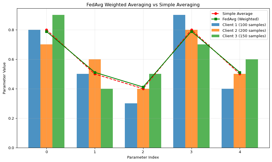
Example 1: FedAvg Weighted Averaging Simulation
This example demonstrates how FedAvg aggregates model weights from multiple clients using weighted averaging based on dataset sizes.
Code
import numpy as npimport matplotlib.pyplot as plt# Simulate client model weights (3 clients, 5 parameters each)client_weights = [ np.array([0.8, 0.5, 0.3, 0.9, 0.4]), # Client 1 np.array([0.7, 0.6, 0.4, 0.8, 0.5]), # Client 2 np.array([0.9, 0.4, 0.5, 0.7, 0.6]) # Client 3]# Dataset sizes for each clientdataset_sizes = np.array([100, 200, 150]) # Total: 450 samples# Simple averaging (incorrect - treats all clients equally)simple_avg = np.mean(client_weights, axis=0)# FedAvg weighted averaging (correct - weights by dataset size)total_samples = np.sum(dataset_sizes)weighted_avg = np.zeros(5)for i, weights inenumerate(client_weights): weight_factor = dataset_sizes[i] / total_samples weighted_avg += weight_factor * weightsprint(f"Client {i+1}: {dataset_sizes[i]} samples ({weight_factor*100:.1f}% weight)")print(f"\nSimple Average: {simple_avg}")print(f"Weighted Average (FedAvg): {weighted_avg}")# Visualize the differencefig, ax = plt.subplots(figsize=(10, 6))x = np.arange(5)width =0.25ax.bar(x - width, client_weights[0], width, label='Client 1 (100 samples)', alpha=0.8)ax.bar(x, client_weights[1], width, label='Client 2 (200 samples)', alpha=0.8)ax.bar(x + width, client_weights[2], width, label='Client 3 (150 samples)', alpha=0.8)ax.plot(x, simple_avg, 'r--', marker='o', label='Simple Average', linewidth=2)ax.plot(x, weighted_avg, 'g-', marker='s', label='FedAvg (Weighted)', linewidth=2)ax.set_xlabel('Parameter Index')ax.set_ylabel('Parameter Value')ax.set_title('FedAvg Weighted Averaging vs Simple Averaging')ax.set_xticks(x)ax.legend()ax.grid(True, alpha=0.3)plt.tight_layout()plt.show()print("\nKey Insight: Client 2 has the most influence (200/450 = 44.4%) because it has")print("the most training data. This prevents bias toward clients with less representative data.")
Client 1: 100 samples (22.2% weight)
Client 2: 200 samples (44.4% weight)
Client 3: 150 samples (33.3% weight)

Simple Average: [0.8 0.5 0.4 0.8 0.5]
Weighted Average (FedAvg): [0.78888889 0.51111111 0.41111111 0.78888889 0.51111111]

Key Insight: Client 2 has the most influence (200/450 = 44.4%) because it has
the most training data. This prevents bias toward clients with less representative data.
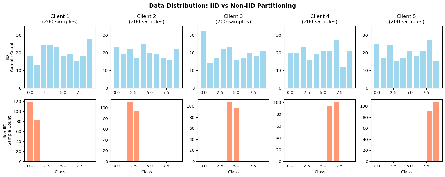
Example 2: IID vs Non-IID Data Partitioning
This example shows how different data partitioning strategies affect federated learning by creating IID and Non-IID distributions.
Code
import numpy as npimport matplotlib.pyplot as plt# Create synthetic dataset (1000 samples, 10 classes)np.random.seed(42)num_samples =1000num_classes =10num_clients =5# Generate labelslabels = np.random.randint(0, num_classes, num_samples)# IID Partitioning: Random uniform splitdef partition_iid(labels, num_clients):"""Each client gets random subset with similar distribution""" indices = np.random.permutation(len(labels)) partition_size =len(labels) // num_clients partitions = []for i inrange(num_clients): start = i * partition_size end = start + partition_size if i < num_clients -1elselen(labels) client_indices = indices[start:end] partitions.append(labels[client_indices])return partitions# Non-IID Partitioning: Label skew (each client gets only 2 classes)def partition_non_iid(labels, num_clients, classes_per_client=2):"""Each client gets only a subset of classes""" partitions = [[] for _ inrange(num_clients)]for client_id inrange(num_clients):# Assign specific classes to this client (rotating) start_class = (client_id * classes_per_client) % num_classes client_classes = [(start_class + i) % num_classes for i inrange(classes_per_client)]for cls in client_classes: class_indices = np.where(labels == cls)[0]# Split class samples among clients that have this class samples_per_client =len(class_indices) // (num_clients // (num_classes // classes_per_client)) start_idx = (client_id % (num_clients // (num_classes // classes_per_client))) * samples_per_client end_idx = start_idx + samples_per_client partitions[client_id].extend(labels[class_indices[start_idx:end_idx]])return [np.array(p) for p in partitions]# Create both partitionsiid_parts = partition_iid(labels, num_clients)non_iid_parts = partition_non_iid(labels, num_clients, classes_per_client=2)# Visualize distributionsfig, axes = plt.subplots(2, num_clients, figsize=(15, 6))for i inrange(num_clients):# IID distribution iid_dist = np.bincount(iid_parts[i], minlength=num_classes) axes[0, i].bar(range(num_classes), iid_dist, color='skyblue', alpha=0.8) axes[0, i].set_title(f'Client {i+1}\n({len(iid_parts[i])} samples)') axes[0, i].set_ylim(0, max([max(np.bincount(p, minlength=num_classes)) for p in iid_parts]) *1.1)if i ==0: axes[0, i].set_ylabel('IID\nSample Count')# Non-IID distribution non_iid_dist = np.bincount(non_iid_parts[i], minlength=num_classes) axes[1, i].bar(range(num_classes), non_iid_dist, color='coral', alpha=0.8) axes[1, i].set_xlabel('Class')if i ==0: axes[1, i].set_ylabel('Non-IID\nSample Count')plt.suptitle('Data Distribution: IID vs Non-IID Partitioning', fontsize=14, fontweight='bold')plt.tight_layout()plt.show()# Calculate entropy (measure of distribution uniformity)def calculate_entropy(partition, num_classes): dist = np.bincount(partition, minlength=num_classes) probs = dist / np.sum(dist) entropy =-np.sum([p * np.log(p +1e-10) for p in probs if p >0])return entropyprint("Entropy Analysis (higher = more uniform distribution):")print(f"Maximum possible entropy: {np.log(num_classes):.3f}")print("\nIID Partitions:")for i, part inenumerate(iid_parts): ent = calculate_entropy(part, num_classes)print(f" Client {i+1}: {ent:.3f} ({ent/np.log(num_classes)*100:.1f}% of max)")print("\nNon-IID Partitions:")for i, part inenumerate(non_iid_parts): ent = calculate_entropy(part, num_classes)print(f" Client {i+1}: {ent:.3f} ({ent/np.log(num_classes)*100:.1f}% of max)")
Entropy Analysis (higher = more uniform distribution):
Maximum possible entropy: 2.303

IID Partitions:
  Client 1: 2.279 (99.0% of max)
  Client 2: 2.293 (99.6% of max)
  Client 3: 2.276 (98.8% of max)
  Client 4: 2.284 (99.2% of max)
  Client 5: 2.282 (99.1% of max)

Non-IID Partitions:
  Client 1: 0.678 (29.4% of max)
  Client 2: 0.690 (30.0% of max)
  Client 3: 0.692 (30.0% of max)
  Client 4: 0.693 (30.1% of max)
  Client 5: 0.690 (30.0% of max)
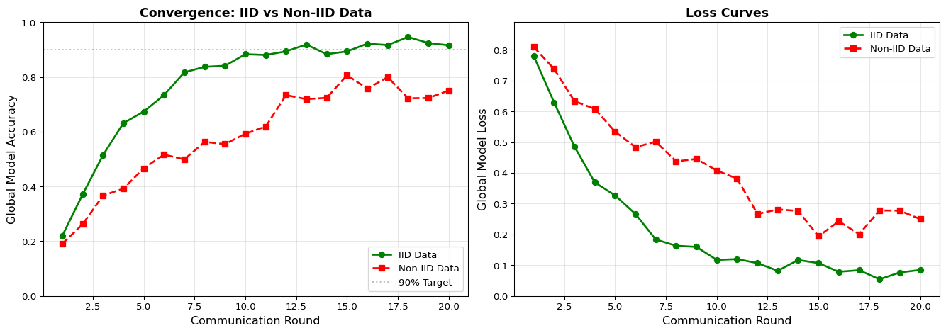
Example 3: Convergence Comparison Visualization
This example simulates and compares the convergence behavior of federated learning with IID vs Non-IID data.
---title: "LAB17: Federated Learning"subtitle: "Distributed Training with Flower"---::: {.callout-note}## PDF Textbook ReferenceFor detailed theoretical foundations, mathematical proofs, and algorithm derivations, see **Chapter 17: Federated Learning with the Flower Framework** in the [PDF textbook](../downloads/Edge-Analytics-Lab-Book-v1.0.0.pdf).The PDF chapter includes:- Complete mathematical foundations of Federated Averaging (FedAvg)- Detailed convergence analysis and communication complexity- In-depth coverage of non-IID data distribution challenges- Comprehensive differential privacy and secure aggregation theory- Theoretical analysis of communication-efficient federated learning:::[](https://colab.research.google.com/github/ngcharithperera/edge-analytics-lab-book/blob/main/notebooks/LAB17_flower_federated.ipynb)[Download Notebook](https://raw.githubusercontent.com/ngcharithperera/edge-analytics-lab-book/main/notebooks/LAB17_flower_federated.ipynb)## Learning ObjectivesBy the end of this lab you should be able to:- Explain the core ideas of federated learning and when it is preferable to centralised training- Implement the FedAvg algorithm using the Flower framework on a simple dataset- Explore the impact of IID vs non-IID client data on convergence and accuracy- Design and run small-scale FL experiments on laptops/Pis that respect edge constraints (bandwidth, memory, energy)## Theory Summary### Why Federated Learning?Traditional machine learning centralizes all training data in one location—a data center or cloud server. Federated Learning (FL) flips this model: **the model travels to the data, not vice versa**.This solves critical problems for edge AI:1. **Privacy**: Raw data never leaves the device (healthcare records, personal photos, typing patterns)2. **Bandwidth**: Sending model updates (KB-MB) is cheaper than sending raw data (GB-TB)3. **Compliance**: GDPR/HIPAA regulations often prohibit centralizing sensitive data4. **Latency**: Local inference with periodically improved global modelsExample: Google's Gboard keyboard learns from your typing patterns via FL—your messages never leave your phone, yet the global model improves from millions of users.### Federated Averaging (FedAvg)FedAvg is the foundational FL algorithm. Each training round:1. **Server broadcasts** current global model weights $w_t$ to selected clients2. **Clients train locally** for $E$ epochs on their private data3. **Clients send back** updated weights $w_i^{t+1}$4. **Server aggregates** via weighted average:$$w_{t+1} = \sum_{i=1}^{K} \frac{n_i}{n} w_i^{t+1}$$where $n_i$ is the number of training samples on client $i$, and $n = \sum n_i$ is the total.**Key insight**: Weighting by sample count ensures clients with more data have proportionally more influence, preventing bias toward smaller datasets.### The Non-IID ChallengeIn real deployments, data is **non-IID** (non-independently and identically distributed). Examples:- Hospital A specializes in cardiology (90% heart patients), Hospital B in pediatrics (90% children)- Smart home users in Alaska vs Florida have vastly different temperature patterns- Mobile keyboards learn from different languages per userNon-IID data causes:- **Slower convergence**: The global model oscillates between different local optima- **Client drift**: Local models diverge, making aggregation less effective- **Accuracy degradation**: The global model may perform poorly on minority data distributionsMitigations: FedProx (adds a regularization term to keep local models close to global), client sampling strategies, or federated data augmentation.## Key Concepts at a Glance::: {.callout-note icon=false}## Core Concepts- **Decentralized Training**: Models train where data lives; only updates travel over the network- **FedAvg Formula**: $w_{new} = \sum_i \frac{n_i}{n} w_i$ (weighted average by sample count)- **Client Fraction**: Percentage of clients selected per round (e.g., $C = 0.1$ = 10%)- **Local Epochs**: Number of epochs each client trains before sending updates ($E = 1-5$ typical)- **Model Consistency**: All clients must use identical architectures—server aggregates by weight position- **IID vs Non-IID**: IID = each client has similar data distribution; Non-IID = skewed/heterogeneous data- **Privacy vs Accuracy**: FL trades some accuracy (vs centralized) for privacy and bandwidth savings:::## Common Pitfalls::: {.callout-warning}## Mistakes to Avoid**Model Architecture Mismatch Between Clients**: The most cryptic FL error. If Client 1 has a 128-neuron layer where Client 2 has 256, aggregation silently produces garbage. **Prevention**: Define the model in one shared file that all clients import. Print `model.summary()` on each client and verify they match exactly.**Training Too Many Local Epochs**: Setting $E = 50$ local epochs causes "client drift"—each client's model wanders far from the global optimum. Start with $E = 1-5$ and increase only if communication is extremely expensive.**Not Weighting by Sample Count**: If you average models without weighting ($w_{new} = \frac{1}{K} \sum w_i$), a client with 10 samples has the same influence as one with 10,000. Always use weighted averaging: `return weights, len(x_train), {}` in Flower's `fit()`.**Forgetting `min_available_clients`**: If your server waits for 10 clients but only 3 connect, training stalls forever. Set `min_available_clients` to the number you actually have for testing, or use `fraction_fit` to select a subset.**Using Different Random Seeds Across Clients**: If clients use different seeds for data shuffling or dropout, models diverge unnecessarily. For reproducibility, set `np.random.seed()` and `tf.random.set_seed()` consistently.**Ignoring Network Failures**: In production FL, clients disconnect mid-round. Flower handles this with timeouts and minimum client requirements, but always test with simulated failures (`client.stop()` or network drops).:::## Quick Reference### Flower Server Setup```pythonimport flwr as flstrategy = fl.server.strategy.FedAvg( fraction_fit=1.0, # Use all available clients per round fraction_evaluate=1.0, # Evaluate on all clients min_fit_clients=3, # Min clients needed to start training min_evaluate_clients=3, # Min clients for evaluation min_available_clients=3, # Wait for this many to connect)fl.server.start_server( server_address="0.0.0.0:8080", config=fl.server.ServerConfig(num_rounds=10), strategy=strategy,)```### Flower Client Implementation```pythonimport flwr as flimport tensorflow as tfclass MNISTClient(fl.client.NumPyClient):def__init__(self, model, x_train, y_train, x_test, y_test):self.model = modelself.x_train, self.y_train = x_train, y_trainself.x_test, self.y_test = x_test, y_testdef get_parameters(self, config):"""Return current model weights"""returnself.model.get_weights()def fit(self, parameters, config):"""Train on local data"""self.model.set_weights(parameters) # Apply global weightsself.model.fit(self.x_train, self.y_train, epochs=1, batch_size=32, verbose=0)returnself.model.get_weights(), len(self.x_train), {} # weights, count, metricsdef evaluate(self, parameters, config):"""Evaluate on local test data"""self.model.set_weights(parameters) loss, accuracy =self.model.evaluate(self.x_test, self.y_test, verbose=0)return loss, len(self.x_test), {"accuracy": accuracy}# Connect to serverfl.client.start_numpy_client( server_address="192.168.1.100:8080", client=MNISTClient(model, x_train, y_train, x_test, y_test))```### Data Partitioning Strategies**IID Partitioning** (random split):```pythondef partition_iid(x_data, y_data, num_clients):"""Random uniform partition""" indices = np.random.permutation(len(x_data)) partition_size =len(x_data) // num_clients partitions = []for i inrange(num_clients): start = i * partition_size end = start + partition_size client_indices = indices[start:end] partitions.append((x_data[client_indices], y_data[client_indices]))return partitions```**Non-IID Partitioning** (label skew):```pythondef partition_non_iid(x_data, y_data, num_clients, classes_per_client=2):"""Each client gets only a subset of classes""" num_classes =len(np.unique(y_data)) partitions = [[] for _ inrange(num_clients)]for client_id inrange(num_clients):# Assign specific classes to this client client_classes = np.random.choice(num_classes, classes_per_client, replace=False)for cls in client_classes: class_indices = np.where(y_data == cls)[0] samples = np.random.choice(class_indices, len(class_indices) // num_clients) partitions[client_id].extend(samples)return [(x_data[indices], y_data[indices]) for indices in partitions]```### FedAvg Hyperparameters| Parameter | Typical Value | Effect | When to Adjust ||-----------|---------------|--------|----------------|| **Rounds** | 10-100 | More rounds = better convergence | Increase for complex tasks || **Local Epochs (E)** | 1-5 | More epochs = less communication | Increase if bandwidth is expensive || **Client Fraction (C)** | 0.1-1.0 | Lower = fewer clients per round | Lower for large deployments (1000+ clients) || **Learning Rate** | 0.001-0.01 | Lower for FL than centralized | Start 10× lower than centralized training || **Batch Size** | 32-64 | Larger = faster but more memory | Reduce for edge devices with limited RAM |### Communication Cost AnalysisFor a model with $M$ parameters (FP32), each round requires:- **Upload per client**: $4M$ bytes (weights)- **Download per client**: $4M$ bytes (global model)- **Total per client**: $8M$ bytes/roundExample: MobileNetV2 (3.5M params) = 14 MB/client/round. With 100 clients and 50 rounds = **70 GB total network traffic**.Compare to centralized training: uploading raw MNIST dataset (60k images × 784 pixels × 1 byte) = **47 MB per client**. FL is more efficient when datasets are large relative to model size.---::: {.callout-tip}## Related Concepts in PDF Chapter 17- Section 17.2: Federated Learning vs traditional centralized training comparison- Section 17.3: FedAvg algorithm mathematical formulation and convergence properties- Section 17.4: Flower framework architecture (server, client, gRPC communication)- Section 17.5: Handling non-IID data with FedProx and client sampling strategies- Section 17.6: Raspberry Pi deployment with multiple networked devices- Section 17.7: Privacy-preserving techniques (secure aggregation, differential privacy):::## Self-Assessment CheckpointsTest your understanding before proceeding to the exercises.::: {.callout-note collapse="true" title="Question 1: Calculate the aggregated weight for 3 clients with weights w1=0.8, w2=0.7, w3=0.9 and dataset sizes n1=100, n2=200, n3=150."}**Answer:** Using FedAvg weighted average: w_global = Σ(n_i / n_total) × w_i. Total samples n = 100 + 200 + 150 = 450. w_global = (100/450)×0.8 + (200/450)×0.7 + (150/450)×0.9 = 0.222×0.8 + 0.444×0.7 + 0.333×0.9 = 0.178 + 0.311 + 0.300 = **0.789**. Client 2 has the most influence (200 samples, 44.4% weight) despite having the lowest individual weight (0.7). This weighting ensures larger datasets don't get drowned out by many small clients. Without weighting (simple average = 0.8), a client with 10 samples would have equal influence to one with 10,000.:::::: {.callout-note collapse="true" title="Question 2: Why does non-IID data slow federated learning convergence compared to IID data?"}**Answer:** **IID data**: Each client has similar data distribution (e.g., all clients see all digit classes 0-9 equally). Local training moves in consistent directions toward the global optimum. Aggregation produces smooth, steady improvement. **Non-IID data**: Client A has mostly 0s and 1s, Client B has mostly 8s and 9s. Client A's local training optimizes for 0/1 classification while destroying performance on 8/9. Client B does the opposite. Aggregation averages these conflicting updates, causing the global model to oscillate and converge slowly or get stuck in poor local minima. Mitigations: (1) **FedProx**: Adds penalty term keeping local models close to global, (2) **Client sampling**: Select diverse clients each round, (3) **More communication rounds**: Compensate for conflicting updates with more averaging.:::::: {.callout-note collapse="true" title="Question 3: Your FL server waits for min_available_clients=10 but only 3 devices connect. What happens and how do you fix it?"}**Answer:** Training stalls forever. The server waits indefinitely for 10 clients but only 3 are available. This is a common deployment issue during development/testing. **Fixes**: (1) **Set min_available_clients=3** to match actual device count, (2) **Use min_fit_clients=2** (minimum to start a round) separately from min_available_clients (wait threshold), (3) **Set timeout** in ServerConfig to start with available clients after waiting, (4) **Use fraction_fit=0.5** to sample 50% of available clients instead of waiting for fixed count. For production: always plan for clients dropping offline—use min_fit_clients = 50-70% of expected to handle network failures gracefully.:::::: {.callout-note collapse="true" title="Question 4: Explain why setting local_epochs=50 causes 'client drift' in federated learning."}**Answer:** **Client drift**: When clients train too many epochs locally, their models wander far from the global model into client-specific local optima. With E=50 local epochs on non-IID data, Client A (heart disease data) optimizes heavily for cardiology features while Client B (pediatrics) optimizes for child-specific patterns. After 50 epochs, their models are so different that aggregation produces an incoherent "average" that performs poorly on both. Result: global model accuracy degrades instead of improving. **Solution**: Keep E=1-5 epochs. The key insight: FL works through frequent communication and averaging, not local perfection. More rounds with less local training (R=100, E=1) beats fewer rounds with heavy training (R=10, E=10) for non-IID data.:::::: {.callout-note collapse="true" title="Question 5: Why is federated learning important for mobile keyboard learning, even though bandwidth savings seem minor?"}**Answer:** It's about **privacy**, not bandwidth. Keyboard learning needs to adapt to your typing patterns, autocorrect preferences, and frequently used words/phrases. Centralizing this data reveals: personal messages, passwords typed, search queries, private conversations, health information, financial data. Even anonymized, typing patterns can identify individuals. **FL solution**: Your phone trains a local model on your typing data. Only model weight updates (KB) are sent to the server—never your actual keystrokes. The global model improves from millions of users while your private data never leaves your device. This is why Google's Gboard, Apple's QuickType, and similar apps use FL: user trust requires privacy guarantees that centralized training cannot provide, even with encryption.:::## Interactive NotebookThe notebook below contains runnable code for all Level 1 activities.{{< embed ../../notebooks/LAB17_flower_federated.ipynb >}}## Three-Tier Activities::: {.panel-tabset}### Level 1: NotebookEnvironment: local Jupyter or Colab, no real network required.Suggested workflow:1. Use the notebook to run Flower-based FL simulations on a single machine: - multiple logical clients (processes) training a shared model (e.g., MNIST).2. Implement at least two partitioning strategies: - IID partitions (each client has a representative slice), - non-IID partitions (each client sees only a subset of labels).3. Record convergence behaviours: - accuracy vs round for IID vs non-IID, - effect of changing local epochs, client fraction, and learning rate.4. Compare final FL performance with a centralised training baseline.### Level 2: SimulatorHere you move beyond single-machine simulation to a “small cluster” on your LAN (or multiple VMs on one host).- Start the Flower server on one machine (or VM).- Run 2–3 clients on other machines/VMs, each with its own data partition.- Use: - **[Our FL Simulator](../simulations/federated-learning.qmd)** to visualise FedAvg behaviour, - **[Flower Documentation](https://flower.ai)** and Colab examples for more complex experiments if desired.- Observe: - how network latency and client dropouts affect round time, - how different choices of client fraction and number of rounds affect convergence.### Level 3: DeviceDeploy an FL experiment to a small Raspberry Pi cluster.1. Choose a simple task (e.g., digit recognition, small sensor-based classifier) and port your client code to Pis.2. Run the Flower server on a laptop/desktop; run clients on 2–3 Pis with local datasets (e.g., different sensors/locations).3. Monitor: - per-round duration and CPU/memory usage on the Pis, - network throughput (roughly how many bytes per round), - convergence behaviour compared with your Level 1/2 experiments.4. Reflect on: - when FL is preferable to centralised training (privacy, bandwidth, regulation), - how FL interacts with LAB18’s on-device learning (per-device adaptation) and LAB15’s energy budget constraints.:::## Related Labs::: {.callout-tip}## Distributed Learning & Privacy- **LAB06: Edge Security** - Privacy and security considerations for FL- **LAB13: Distributed Data** - Distributed data management systems- **LAB18: On-Device Learning** - Compare with local adaptation strategies:::::: {.callout-tip}## Foundation & Optimization- **LAB02: ML Foundations** - Training basics before distributed training- **LAB03: Quantization** - Optimize models for FL clients- **LAB15: Energy Optimization** - Energy-efficient distributed training:::## Try It Yourself: Executable Python ExamplesThe following code blocks are fully executable and demonstrate key federated learning concepts. Each example is self-contained and can be run directly in this Quarto document.### Example 1: FedAvg Weighted Averaging SimulationThis example demonstrates how FedAvg aggregates model weights from multiple clients using weighted averaging based on dataset sizes.```{python}import numpy as npimport matplotlib.pyplot as plt# Simulate client model weights (3 clients, 5 parameters each)client_weights = [ np.array([0.8, 0.5, 0.3, 0.9, 0.4]), # Client 1 np.array([0.7, 0.6, 0.4, 0.8, 0.5]), # Client 2 np.array([0.9, 0.4, 0.5, 0.7, 0.6]) # Client 3]# Dataset sizes for each clientdataset_sizes = np.array([100, 200, 150]) # Total: 450 samples# Simple averaging (incorrect - treats all clients equally)simple_avg = np.mean(client_weights, axis=0)# FedAvg weighted averaging (correct - weights by dataset size)total_samples = np.sum(dataset_sizes)weighted_avg = np.zeros(5)for i, weights inenumerate(client_weights): weight_factor = dataset_sizes[i] / total_samples weighted_avg += weight_factor * weightsprint(f"Client {i+1}: {dataset_sizes[i]} samples ({weight_factor*100:.1f}% weight)")print(f"\nSimple Average: {simple_avg}")print(f"Weighted Average (FedAvg): {weighted_avg}")# Visualize the differencefig, ax = plt.subplots(figsize=(10, 6))x = np.arange(5)width =0.25ax.bar(x - width, client_weights[0], width, label='Client 1 (100 samples)', alpha=0.8)ax.bar(x, client_weights[1], width, label='Client 2 (200 samples)', alpha=0.8)ax.bar(x + width, client_weights[2], width, label='Client 3 (150 samples)', alpha=0.8)ax.plot(x, simple_avg, 'r--', marker='o', label='Simple Average', linewidth=2)ax.plot(x, weighted_avg, 'g-', marker='s', label='FedAvg (Weighted)', linewidth=2)ax.set_xlabel('Parameter Index')ax.set_ylabel('Parameter Value')ax.set_title('FedAvg Weighted Averaging vs Simple Averaging')ax.set_xticks(x)ax.legend()ax.grid(True, alpha=0.3)plt.tight_layout()plt.show()print("\nKey Insight: Client 2 has the most influence (200/450 = 44.4%) because it has")print("the most training data. This prevents bias toward clients with less representative data.")```### Example 2: IID vs Non-IID Data PartitioningThis example shows how different data partitioning strategies affect federated learning by creating IID and Non-IID distributions.```{python}import numpy as npimport matplotlib.pyplot as plt# Create synthetic dataset (1000 samples, 10 classes)np.random.seed(42)num_samples =1000num_classes =10num_clients =5# Generate labelslabels = np.random.randint(0, num_classes, num_samples)# IID Partitioning: Random uniform splitdef partition_iid(labels, num_clients):"""Each client gets random subset with similar distribution""" indices = np.random.permutation(len(labels)) partition_size =len(labels) // num_clients partitions = []for i inrange(num_clients): start = i * partition_size end = start + partition_size if i < num_clients -1elselen(labels) client_indices = indices[start:end] partitions.append(labels[client_indices])return partitions# Non-IID Partitioning: Label skew (each client gets only 2 classes)def partition_non_iid(labels, num_clients, classes_per_client=2):"""Each client gets only a subset of classes""" partitions = [[] for _ inrange(num_clients)]for client_id inrange(num_clients):# Assign specific classes to this client (rotating) start_class = (client_id * classes_per_client) % num_classes client_classes = [(start_class + i) % num_classes for i inrange(classes_per_client)]for cls in client_classes: class_indices = np.where(labels == cls)[0]# Split class samples among clients that have this class samples_per_client =len(class_indices) // (num_clients // (num_classes // classes_per_client)) start_idx = (client_id % (num_clients // (num_classes // classes_per_client))) * samples_per_client end_idx = start_idx + samples_per_client partitions[client_id].extend(labels[class_indices[start_idx:end_idx]])return [np.array(p) for p in partitions]# Create both partitionsiid_parts = partition_iid(labels, num_clients)non_iid_parts = partition_non_iid(labels, num_clients, classes_per_client=2)# Visualize distributionsfig, axes = plt.subplots(2, num_clients, figsize=(15, 6))for i inrange(num_clients):# IID distribution iid_dist = np.bincount(iid_parts[i], minlength=num_classes) axes[0, i].bar(range(num_classes), iid_dist, color='skyblue', alpha=0.8) axes[0, i].set_title(f'Client {i+1}\n({len(iid_parts[i])} samples)') axes[0, i].set_ylim(0, max([max(np.bincount(p, minlength=num_classes)) for p in iid_parts]) *1.1)if i ==0: axes[0, i].set_ylabel('IID\nSample Count')# Non-IID distribution non_iid_dist = np.bincount(non_iid_parts[i], minlength=num_classes) axes[1, i].bar(range(num_classes), non_iid_dist, color='coral', alpha=0.8) axes[1, i].set_xlabel('Class')if i ==0: axes[1, i].set_ylabel('Non-IID\nSample Count')plt.suptitle('Data Distribution: IID vs Non-IID Partitioning', fontsize=14, fontweight='bold')plt.tight_layout()plt.show()# Calculate entropy (measure of distribution uniformity)def calculate_entropy(partition, num_classes): dist = np.bincount(partition, minlength=num_classes) probs = dist / np.sum(dist) entropy =-np.sum([p * np.log(p +1e-10) for p in probs if p >0])return entropyprint("Entropy Analysis (higher = more uniform distribution):")print(f"Maximum possible entropy: {np.log(num_classes):.3f}")print("\nIID Partitions:")for i, part inenumerate(iid_parts): ent = calculate_entropy(part, num_classes)print(f" Client {i+1}: {ent:.3f} ({ent/np.log(num_classes)*100:.1f}% of max)")print("\nNon-IID Partitions:")for i, part inenumerate(non_iid_parts): ent = calculate_entropy(part, num_classes)print(f" Client {i+1}: {ent:.3f} ({ent/np.log(num_classes)*100:.1f}% of max)")```### Example 3: Convergence Comparison VisualizationThis example simulates and compares the convergence behavior of federated learning with IID vs Non-IID data.```{python}import numpy as npimport matplotlib.pyplot as pltnp.random.seed(42)# Simulation parametersnum_rounds =20num_clients =5# Simulate convergence for IID datadef simulate_convergence_iid(num_rounds, base_acc=0.95, noise_level=0.02):"""Simulate smooth convergence with IID data""" rounds = np.arange(1, num_rounds +1)# Fast exponential convergence accuracy = base_acc * (1- np.exp(-rounds /4))# Add small random noise accuracy += np.random.normal(0, noise_level, num_rounds) accuracy = np.clip(accuracy, 0, 1)return rounds, accuracy# Simulate convergence for Non-IID datadef simulate_convergence_non_iid(num_rounds, base_acc=0.95, degradation=0.15, noise_level=0.03):"""Simulate slower, oscillating convergence with Non-IID data""" rounds = np.arange(1, num_rounds +1)# Slower convergence with accuracy penalty accuracy = (base_acc - degradation) * (1- np.exp(-rounds /6))# Add oscillation due to client drift accuracy +=0.05* np.sin(rounds /2)# Add larger noise accuracy += np.random.normal(0, noise_level, num_rounds) accuracy = np.clip(accuracy, 0, 1)return rounds, accuracy# Generate convergence curvesrounds_iid, acc_iid = simulate_convergence_iid(num_rounds)rounds_non_iid, acc_non_iid = simulate_convergence_non_iid(num_rounds)# Calculate loss (inverse of accuracy for visualization)loss_iid =1- acc_iidloss_non_iid =1- acc_non_iid# Visualizationfig, axes = plt.subplots(1, 2, figsize=(14, 5))# Accuracy comparisonaxes[0].plot(rounds_iid, acc_iid, 'g-', marker='o', label='IID Data', linewidth=2, markersize=6)axes[0].plot(rounds_non_iid, acc_non_iid, 'r--', marker='s', label='Non-IID Data', linewidth=2, markersize=6)axes[0].axhline(y=0.9, color='gray', linestyle=':', alpha=0.5, label='90% Target')axes[0].set_xlabel('Communication Round', fontsize=12)axes[0].set_ylabel('Global Model Accuracy', fontsize=12)axes[0].set_title('Convergence: IID vs Non-IID Data', fontsize=13, fontweight='bold')axes[0].legend(loc='lower right')axes[0].grid(True, alpha=0.3)axes[0].set_ylim(0, 1)# Loss comparisonaxes[1].plot(rounds_iid, loss_iid, 'g-', marker='o', label='IID Data', linewidth=2, markersize=6)axes[1].plot(rounds_non_iid, loss_non_iid, 'r--', marker='s', label='Non-IID Data', linewidth=2, markersize=6)axes[1].set_xlabel('Communication Round', fontsize=12)axes[1].set_ylabel('Global Model Loss', fontsize=12)axes[1].set_title('Loss Curves', fontsize=13, fontweight='bold')axes[1].legend(loc='upper right')axes[1].grid(True, alpha=0.3)axes[1].set_ylim(0, max(loss_iid.max(), loss_non_iid.max()) *1.1)plt.tight_layout()plt.show()# Performance metricsprint("Performance Comparison:")print(f"\nIID Data:")print(f" Final Accuracy: {acc_iid[-1]:.2%}")print(f" Rounds to 90%: {np.argmax(acc_iid >=0.9) +1ifany(acc_iid >=0.9) else'Not reached'}")print(f" Convergence Rate: Fast (smooth exponential)")print(f"\nNon-IID Data:")print(f" Final Accuracy: {acc_non_iid[-1]:.2%}")print(f" Rounds to 90%: {np.argmax(acc_non_iid >=0.9) +1ifany(acc_non_iid >=0.9) else'Not reached'}")print(f" Convergence Rate: Slow (oscillating, client drift)")degradation = (acc_iid[-1] - acc_non_iid[-1]) / acc_iid[-1] *100print(f"\nAccuracy Degradation: {degradation:.1f}%")print(f"Additional rounds needed: ~{int((num_rounds * degradation) /100)}")```### Example 4: Privacy Budget DemonstrationThis example demonstrates the privacy-utility tradeoff in differential privacy for federated learning.```{python}import numpy as npimport matplotlib.pyplot as pltnp.random.seed(42)# Privacy parametersepsilon_values = [0.1, 0.5, 1.0, 5.0, 10.0, 100.0] # Privacy budgetsdelta =1e-5sensitivity =1.0# Maximum L2 norm of gradientsdef calculate_noise_scale(epsilon, delta, sensitivity):"""Calculate Gaussian noise scale for (ε, δ)-differential privacy"""return sensitivity * np.sqrt(2* np.log(1.25/ delta)) / epsilondef simulate_dp_training(epsilon, base_accuracy=0.95):"""Simulate how DP noise affects model accuracy"""# Privacy-utility tradeoff: lower epsilon = more noise = lower accuracy noise_scale = calculate_noise_scale(epsilon, delta, sensitivity)# Model accuracy decreases with more noise (lower epsilon) privacy_penalty =1.0/ (1.0+ epsilon) final_accuracy = base_accuracy * (1-0.3* privacy_penalty)return final_accuracy, noise_scale# Calculate accuracy for different privacy budgetsresults = []for eps in epsilon_values: acc, noise = simulate_dp_training(eps) privacy_level ='High'if eps <1.0else ('Medium'if eps <5.0else'Low') results.append({'epsilon': eps,'accuracy': acc,'noise_scale': noise,'privacy_level': privacy_level })# Visualizationfig, axes = plt.subplots(1, 2, figsize=(14, 5))# Privacy-Utility Tradeoffepsilons = [r['epsilon'] for r in results]accuracies = [r['accuracy'] for r in results]axes[0].semilogx(epsilons, accuracies, 'bo-', linewidth=2, markersize=8)axes[0].axhline(y=0.95, color='green', linestyle='--', alpha=0.5, label='No Privacy (95%)')axes[0].axvline(x=1.0, color='orange', linestyle=':', alpha=0.5, label='ε=1 (Strong Privacy)')axes[0].set_xlabel('Privacy Budget (ε)', fontsize=12)axes[0].set_ylabel('Model Accuracy', fontsize=12)axes[0].set_title('Privacy-Utility Tradeoff', fontsize=13, fontweight='bold')axes[0].grid(True, alpha=0.3)axes[0].legend()# Add privacy zone shadingaxes[0].axvspan(0, 1, alpha=0.1, color='green', label='High Privacy')axes[0].axvspan(1, 5, alpha=0.1, color='yellow')axes[0].axvspan(5, 100, alpha=0.1, color='red')# Noise scale vs epsilonnoise_scales = [r['noise_scale'] for r in results]axes[1].loglog(epsilons, noise_scales, 'rs-', linewidth=2, markersize=8)axes[1].set_xlabel('Privacy Budget (ε)', fontsize=12)axes[1].set_ylabel('Noise Scale (σ)', fontsize=12)axes[1].set_title('Gaussian Noise Scale vs Privacy Budget', fontsize=13, fontweight='bold')axes[1].grid(True, alpha=0.3, which='both')plt.tight_layout()plt.show()# Summary tableprint("\nPrivacy-Utility Analysis")print("="*80)print(f"{'Epsilon':<10}{'Privacy':<15}{'Accuracy':<12}{'Noise Scale':<15}{'Use Case'}")print("-"*80)for r in results:if r['epsilon'] <=1.0: use_case ="Medical/Financial"elif r['epsilon'] <=5.0: use_case ="General Apps"else: use_case ="Low-risk Apps"print(f"{r['epsilon']:<10.1f}{r['privacy_level']:<15}{r['accuracy']:<12.1%} "f"{r['noise_scale']:<15.4f}{use_case}")print("\nKey Insights:")print(f"• ε < 1: Strong privacy guarantee, but accuracy drops by ~{(0.95-results[0]['accuracy'])*100:.1f}%")print(f"• ε = 1: Good balance - commonly used for sensitive applications")print(f"• ε > 10: Weak privacy, minimal accuracy impact")print(f"• Lower ε → Higher noise → More privacy → Lower utility")```## Related Resources- [Hardware Guide](../resources/hardware.qmd) - Equipment needed for Level 3- [Troubleshooting](../resources/troubleshooting.qmd) - Common issues and solutions