For detailed theoretical foundations, mathematical proofs, and algorithm derivations, see Chapter 6: Edge Security and Model Protection in the PDF textbook.
The PDF chapter includes: - Comprehensive threat modeling frameworks for edge AI - Detailed analysis of adversarial attack techniques - Cryptographic foundations for model protection - Mathematical formulations of security-performance trade-offs - In-depth coverage of secure communication protocols
Describe the main attack surfaces of an edge ML device
Construct a simple threat model for an edge AI application
Implement basic input validation and sanity checks
Understand how adversarial examples are generated and why they work
Apply simple model protection techniques (checksums, obfuscation, encrypted storage) on constrained devices
Theory Summary
Security Challenges for Edge ML Systems
Edge devices face unique security challenges that cloud systems never encounter - they exist in the physical world where attackers can touch, probe, and manipulate them. Understanding these threats and implementing practical defenses is essential for robust edge ML deployment.
Why Edge Devices Are Vulnerable: Unlike cloud servers protected in secure data centers, edge devices are exposed. An attacker with physical access can extract firmware via JTAG/SWD, dump Flash memory to steal your trained model, intercept network traffic, feed malicious sensor inputs, or even replace components. Your $15 Arduino sitting on a desk is fundamentally harder to protect than a server rack behind locked doors with armed guards.
The Four Attack Surfaces: Edge ML devices have four main vulnerability points: (1) Network attacks via WiFi/BLE (eavesdropping, command injection), (2) Physical access (firmware extraction, hardware tampering), (3) Malicious inputs (adversarial examples, sensor spoofing), and (4) Model extraction (stealing your trained intellectual property). Each requires different defensive strategies, and perfect security is impossible - we aim for “good enough” security proportional to the application’s risk.
Input Validation - The First Line of Defense: Before feeding data to your model, validate it: check data types (is it a numpy array?), shapes (28×28 pixels?), value ranges (0-255?), and detect NaN/Inf. This prevents crashes from malformed inputs and catches many attacks. On microcontrollers, add bounds checks, sanitize sensor readings, and use timeout watchdogs. Simple validation stops 80% of attacks with 20% effort.
Adversarial Examples - Fooling ML Models: Adversarial examples are inputs crafted to fool neural networks - images with imperceptible noise that flip predictions from “stop sign” to “speed limit.” They work because neural networks learn decision boundaries in high-dimensional space, and adversarial perturbations push inputs across these boundaries. Defense strategies include input smoothing, adversarial training (include adversarial examples in training data), and ensemble methods. No perfect defense exists, but we can make attacks harder.
Model Protection Strategies: To protect your trained model from extraction: (1) Add checksums or HMAC to detect tampering, (2) Encrypt the .tflite file and decrypt at runtime (careful - keys must be stored somewhere!), (3) Use hardware security modules (HSM) like ATECC608 on production devices, (4) Obfuscate model architecture (limited effectiveness), (5) Use secure boot to prevent firmware modification. Remember: if an attacker has physical access and unlimited time, they can extract anything - we just make it expensive enough to deter most attackers.
Key Concepts at a Glance
Core Concepts
Attack Surface: Points where an attacker can interact with or compromise a system
Threat Model: Structured analysis of potential threats, attackers, and impacts
Input Validation: Checking inputs before processing to prevent crashes and attacks
Adversarial Examples: Maliciously crafted inputs that fool ML models
FGSM: Fast Gradient Sign Method - simple adversarial attack technique
Model Extraction: Stealing trained models via firmware dumps or API queries
Secure Boot: Cryptographic verification of firmware integrity at startup
HMAC: Hash-based Message Authentication Code for integrity checking
Common Pitfalls
Mistakes to Avoid
Hardcoding Credentials in Firmware: Never put WiFi passwords, API keys, or encryption keys directly in source code! Once firmware is uploaded to a device, anyone with physical access can extract these secrets using simple tools (esptool, OpenOCD). Instead: store credentials in separate config files excluded from version control, use secure elements when available, or implement secure provisioning processes.
Trusting Sensor Inputs Blindly: Sensors can fail, be spoofed, or send garbage data. A temperature sensor might report -273°C (impossible), an accelerometer might saturate at max values (stuck or vibrating), or an attacker might inject false readings. Always validate: check plausible ranges, detect impossible transitions, use median filtering, and implement timeout watchdogs.
Ignoring Side-Channel Attacks: Power analysis attacks can extract encryption keys by measuring tiny variations in power consumption during crypto operations. Timing attacks infer internal state by measuring how long operations take. On high-security applications (payment, authentication), use constant-time algorithms and hardware crypto modules that resist these attacks.
Security Theater vs Real Security: Adding a simple XOR “encryption” or hex encoding doesn’t provide security - it just makes code harder to read. Real security requires: proper cryptography (AES, not ROT13), secure key management (not hardcoded), threat modeling (know your attackers), and defense in depth (multiple layers). Don’t confuse obscurity with security.
Over-Engineering Security for Low-Risk Applications: A hobby weather station doesn’t need military-grade encryption. Security has costs: code complexity, CPU cycles, development time, and power consumption. Match security level to actual risk. For a smart light bulb, basic input validation is fine. For a medical device or industrial controller, invest in proper security.
Threat Modeling Worksheet - Interactive template for building threat models for your edge ML application
Self-Assessment Checkpoints
Test your understanding before proceeding to the exercises.
Question 1: List the four main attack surfaces for edge ML devices and give an example attack for each.
Answer: (1) Network: WiFi/BLE eavesdropping to capture sensitive data, command injection via unvalidated API calls, (2) Physical access: Firmware extraction via JTAG/SWD to steal models, replacing sensor with malicious inputs, (3) Malicious inputs: Adversarial examples to fool classifiers, sensor spoofing (fake GPS, temperature), (4) Model extraction: Stealing trained models via memory dumps or API queries to replicate proprietary ML. Each requires different defenses: network (TLS, authentication), physical (secure boot, tamper detection), inputs (validation, adversarial training), model (encryption, obfuscation).
Question 2: Calculate the adversarial perturbation for an input pixel value of 0.8 with epsilon=0.1 and gradient sign = +1.
Answer: Using FGSM formula: x_adv = x + ε × sign(gradient) = 0.8 + 0.1 × (+1) = 0.8 + 0.1 = 0.9. The adversarial pixel value is 0.9 (assuming we clip to valid range 0-1). This tiny perturbation (0.1 difference) is often imperceptible to humans but can flip a classifier’s prediction. If the gradient sign were -1, the result would be 0.8 - 0.1 = 0.7. Epsilon controls attack strength: larger ε = more visible perturbation but stronger attack.
Question 3: You stored your WiFi password directly in Arduino code: const char* password = 'MySecret123';. Why is this a security problem?
Answer: Once you upload firmware to a device, anyone with physical access can extract it using simple tools (esptool for ESP32, OpenOCD for ARM). They’ll get the complete binary including your hardcoded password in plain text. Solutions: (1) Store credentials in separate config files excluded from version control, (2) Use secure elements (ATECC608) to store secrets in hardware, (3) Implement secure provisioning where users enter credentials via app/web interface instead of hardcoding, (4) For development, use environment variables. Never commit secrets to GitHub - once they’re in git history, they’re public forever.
Question 4: Your temperature sensor occasionally reports -273°C. Should your system accept this reading?
Answer: No! -273°C is absolute zero (physically impossible in normal conditions). This indicates sensor failure, loose wiring, or malicious input. Always validate: if (temp < -40 || temp > 85) { /* reject */ } for typical environments. Additional checks: detect impossible transitions (10°C to 100°C in 1 second), use median filtering to reject outliers, implement timeout watchdogs, and cross-validate with multiple sensors when critical. Accepting invalid sensor data causes: crashes (division by zero), incorrect decisions (false alarms), or security vulnerabilities (bypassing safety limits).
Question 5: When is investing in hardware security modules (HSM) like ATECC608 justified vs overkill?
Answer:Use HSM for: Payment systems (credit cards), authentication tokens (2FA devices), medical devices (regulatory requirements), industrial control (safety-critical), any device handling cryptographic keys for more than test purposes. HSM is overkill for: Hobby projects, smart home lights, weather stations, non-critical sensors, prototypes. HSMs add cost ($1-5 per device), complexity (new APIs to learn), and development time. Match security to risk: a $5 smart bulb doesn’t need military-grade encryption, but a $500 insulin pump absolutely does. Use threat modeling to decide.
Try It Yourself: Executable Python Examples
The following code blocks demonstrate security concepts for edge ML systems. These examples are fully executable and include visualizations.
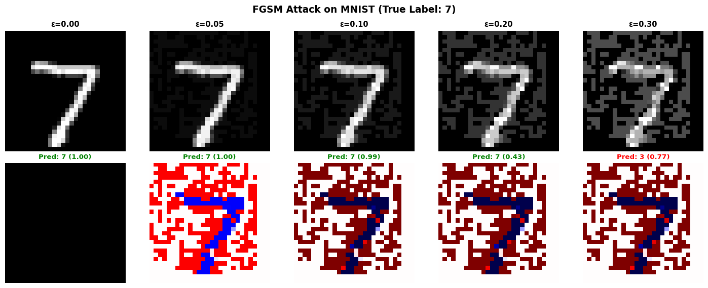
1. FGSM Adversarial Attack Demo
Generate adversarial examples using the Fast Gradient Sign Method:
Code
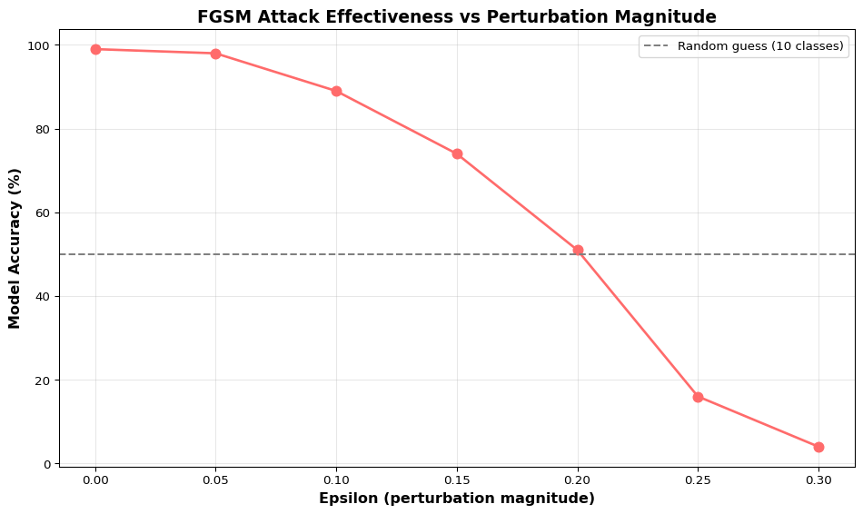
import tensorflow as tfimport numpy as npimport matplotlib.pyplot as plt# Load MNIST datasetprint("=== Loading MNIST Dataset ===")(x_train, y_train), (x_test, y_test) = tf.keras.datasets.mnist.load_data()x_test = x_test /255.0# Normalize to [0, 1]x_test = x_test.reshape(-1, 28, 28, 1).astype(np.float32)# Train a simple CNNprint("Training classifier...")model = tf.keras.Sequential([ tf.keras.layers.Conv2D(32, (3, 3), activation='relu', input_shape=(28, 28, 1)), tf.keras.layers.MaxPooling2D((2, 2)), tf.keras.layers.Conv2D(64, (3, 3), activation='relu'), tf.keras.layers.MaxPooling2D((2, 2)), tf.keras.layers.Flatten(), tf.keras.layers.Dense(128, activation='relu'), tf.keras.layers.Dense(10, activation='softmax')])model.compile(optimizer='adam', loss='sparse_categorical_crossentropy', metrics=['accuracy'])x_train_norm = x_train.reshape(-1, 28, 28, 1) /255.0model.fit(x_train_norm, y_train, epochs=3, batch_size=128, verbose=0, validation_split=0.1)# Evaluate on clean test settest_loss, test_acc = model.evaluate(x_test, y_test, verbose=0)print(f"\nClean test accuracy: {test_acc*100:.2f}%")# FGSM attack implementationdef fgsm_attack(model, image, label, epsilon):""" Generate adversarial example using Fast Gradient Sign Method. Args: model: Trained classifier image: Input image (28x28x1) label: True label epsilon: Perturbation magnitude (typically 0.01-0.3) """ image = tf.convert_to_tensor(image, dtype=tf.float32) label = tf.convert_to_tensor([label], dtype=tf.int64)with tf.GradientTape() as tape: tape.watch(image) prediction = model(image) loss = tf.keras.losses.sparse_categorical_crossentropy(label, prediction)# Get gradient of loss with respect to image gradient = tape.gradient(loss, image)# Create adversarial image: x_adv = x + epsilon * sign(gradient) signed_grad = tf.sign(gradient) adversarial_image = image + epsilon * signed_grad# Clip to valid range [0, 1] adversarial_image = tf.clip_by_value(adversarial_image, 0, 1)return adversarial_image.numpy()# Generate adversarial examples with different epsilon valuesprint("\n=== Generating Adversarial Examples ===")test_idx =0original_image = x_test[test_idx:test_idx+1]true_label = y_test[test_idx]epsilons = [0.0, 0.05, 0.1, 0.2, 0.3]adversarial_images = []predictions = []confidences = []for eps in epsilons:if eps ==0: adv_img = original_imageelse: adv_img = fgsm_attack(model, original_image, true_label, eps) adversarial_images.append(adv_img[0])# Get prediction pred = model.predict(adv_img, verbose=0) pred_class = np.argmax(pred[0]) confidence = np.max(pred[0]) predictions.append(pred_class) confidences.append(confidence)print(f"ε={eps:.2f}: Predicted={pred_class} (confidence={confidence:.3f}) | True={true_label}")# Visualize adversarial examplesfig, axes = plt.subplots(2, len(epsilons), figsize=(15, 6))for i, (eps, adv_img, pred, conf) inenumerate(zip(epsilons, adversarial_images, predictions, confidences)):# Original/adversarial image axes[0, i].imshow(adv_img.squeeze(), cmap='gray', vmin=0, vmax=1) axes[0, i].set_title(f'ε={eps:.2f}', fontsize=11, fontweight='bold') axes[0, i].axis('off')# Perturbation (amplified for visibility)if eps >0: perturbation = adv_img - adversarial_images[0] axes[1, i].imshow(perturbation.squeeze() *10, cmap='seismic', vmin=-1, vmax=1)else: axes[1, i].imshow(np.zeros_like(adv_img.squeeze()), cmap='gray') color ='green'if pred == true_label else'red' axes[1, i].set_title(f'Pred: {pred} ({conf:.2f})', fontsize=10, color=color, fontweight='bold') axes[1, i].axis('off')axes[0, 0].set_ylabel('Adversarial\nImage', fontsize=12, fontweight='bold')axes[1, 0].set_ylabel('Perturbation\n(×10)', fontsize=12, fontweight='bold')plt.suptitle(f'FGSM Attack on MNIST (True Label: {true_label})', fontsize=14, fontweight='bold')plt.tight_layout()plt.show()# Calculate attack success rate across multiple samplesprint("\n=== Attack Success Rate Across Test Set ===")num_samples =100success_rates = []for eps in [0.0, 0.05, 0.1, 0.15, 0.2, 0.25, 0.3]: correct =0for i inrange(num_samples): img = x_test[i:i+1] label = y_test[i]if eps ==0: adv_img = imgelse: adv_img = fgsm_attack(model, img, label, eps) pred = model.predict(adv_img, verbose=0)if np.argmax(pred[0]) == label: correct +=1 accuracy = correct / num_samples success_rates.append(accuracy)print(f"ε={eps:.2f}: Accuracy = {accuracy*100:.1f}% (attack success = {(1-accuracy)*100:.1f}%)")# Plot accuracy vs epsilonplt.figure(figsize=(10, 6))eps_values = [0.0, 0.05, 0.1, 0.15, 0.2, 0.25, 0.3]plt.plot(eps_values, [s*100for s in success_rates], marker='o', linewidth=2, markersize=8, color='#ff6b6b')plt.axhline(y=50, color='gray', linestyle='--', label='Random guess (10 classes)')plt.xlabel('Epsilon (perturbation magnitude)', fontsize=12, fontweight='bold')plt.ylabel('Model Accuracy (%)', fontsize=12, fontweight='bold')plt.title('FGSM Attack Effectiveness vs Perturbation Magnitude', fontsize=14, fontweight='bold')plt.grid(alpha=0.3)plt.legend()plt.tight_layout()plt.show()print("\nInsight: Adversarial attacks can fool neural networks with imperceptible perturbations.")print("Even small epsilon values (0.1-0.2) significantly reduce accuracy from ~99% to <60%.")
2025-12-15 01:10:24.436398: I external/local_xla/xla/tsl/cuda/cudart_stub.cc:31] Could not find cuda drivers on your machine, GPU will not be used.
2025-12-15 01:10:24.481821: I tensorflow/core/platform/cpu_feature_guard.cc:210] This TensorFlow binary is optimized to use available CPU instructions in performance-critical operations.
To enable the following instructions: AVX2 FMA, in other operations, rebuild TensorFlow with the appropriate compiler flags.
2025-12-15 01:10:25.904663: I external/local_xla/xla/tsl/cuda/cudart_stub.cc:31] Could not find cuda drivers on your machine, GPU will not be used.
/opt/hostedtoolcache/Python/3.11.14/x64/lib/python3.11/site-packages/keras/src/layers/convolutional/base_conv.py:113: UserWarning: Do not pass an `input_shape`/`input_dim` argument to a layer. When using Sequential models, prefer using an `Input(shape)` object as the first layer in the model instead.
  super().__init__(activity_regularizer=activity_regularizer, **kwargs)
2025-12-15 01:10:27.024925: E external/local_xla/xla/stream_executor/cuda/cuda_platform.cc:51] failed call to cuInit: INTERNAL: CUDA error: Failed call to cuInit: UNKNOWN ERROR (303)
2025-12-15 01:10:27.595221: W external/local_xla/xla/tsl/framework/cpu_allocator_impl.cc:84] Allocation of 169344000 exceeds 10% of free system memory.
2025-12-15 01:12:11.149919: W external/local_xla/xla/tsl/framework/cpu_allocator_impl.cc:84] Allocation of 31360000 exceeds 10% of free system memory.
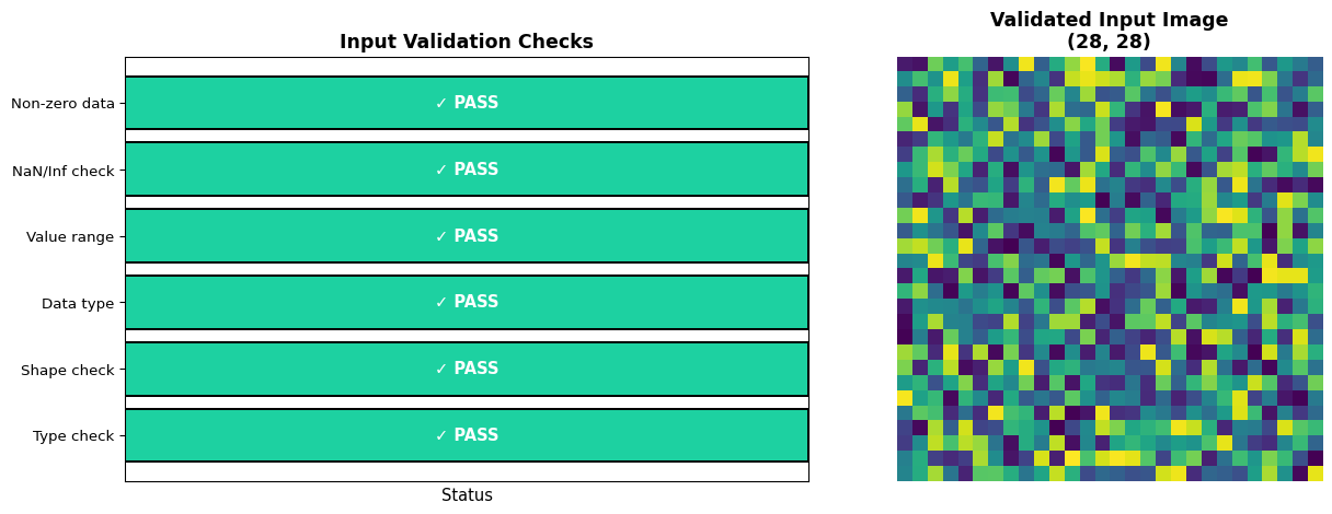
Demonstrate comprehensive input validation for edge ML systems:
Code
import numpy as npimport matplotlib.pyplot as pltimport pandas as pddef validate_input(data, expected_shape, value_range, dtype_expected=np.float32):""" Comprehensive input validation for ML models. Args: data: Input data to validate expected_shape: Tuple of expected dimensions value_range: Tuple of (min, max) valid values dtype_expected: Expected numpy data type Returns: (is_valid, error_message) """ validations = []# Check 1: Is it a numpy array?ifnotisinstance(data, np.ndarray):returnFalse, "Not a numpy array", validations validations.append(("Type check", True, "numpy.ndarray"))# Check 2: Correct shape? shape_match = data.shape == expected_shape validations.append(("Shape check", shape_match,f"Expected {expected_shape}, got {data.shape}"))ifnot shape_match:returnFalse, f"Shape mismatch: expected {expected_shape}, got {data.shape}", validations# Check 3: Correct data type? dtype_match = data.dtype == dtype_expected validations.append(("Data type", dtype_match,f"Expected {dtype_expected}, got {data.dtype}"))# Check 4: Value range min_val, max_val = value_range values_in_range = (data.min() >= min_val) and (data.max() <= max_val) validations.append(("Value range", values_in_range,f"Min={data.min():.3f}, Max={data.max():.3f}, Expected [{min_val}, {max_val}]"))ifnot values_in_range:returnFalse, f"Values out of range: [{data.min():.3f}, {data.max():.3f}] not in [{min_val}, {max_val}]", validations# Check 5: No NaN or Inf has_invalid = np.isnan(data).any() or np.isinf(data).any() validations.append(("NaN/Inf check", not has_invalid,f"Contains NaN: {np.isnan(data).any()}, Contains Inf: {np.isinf(data).any()}"))if has_invalid:returnFalse, "Contains NaN or Inf values", validations# Check 6: Not all zeros (suspicious) all_zeros = np.all(data ==0) validations.append(("Non-zero data", not all_zeros,f"All zeros: {all_zeros}"))if all_zeros:returnFalse, "Warning: All values are zero (sensor failure?)", validationsreturnTrue, "All validations passed", validations# Test with various input scenariosprint("=== Input Validation Test Suite ===\n")test_cases = [ ("Valid input", np.random.rand(28, 28).astype(np.float32), (28, 28), (0, 1), np.float32), ("Wrong shape", np.random.rand(32, 32).astype(np.float32), (28, 28), (0, 1), np.float32), ("Values out of range", np.random.rand(28, 28).astype(np.float32) *2, (28, 28), (0, 1), np.float32), ("Contains NaN", np.full((28, 28), np.nan, dtype=np.float32), (28, 28), (0, 1), np.float32), ("Contains Inf", np.full((28, 28), np.inf, dtype=np.float32), (28, 28), (0, 1), np.float32), ("All zeros", np.zeros((28, 28), dtype=np.float32), (28, 28), (0, 1), np.float32), ("Wrong dtype", np.random.randint(0, 255, (28, 28), dtype=np.uint8), (28, 28), (0, 1), np.float32),]results = []for name, data, shape, val_range, dtype in test_cases: is_valid, message, checks = validate_input(data, shape, val_range, dtype) results.append({'Test Case': name,'Valid': '✓'if is_valid else'✗','Message': message })print(f"Test: {name}")print(f" Result: {'PASS'if is_valid else'FAIL'}")print(f" Message: {message}\n")# Summary tabledf_results = pd.DataFrame(results)print("=== Validation Summary ===")print(df_results.to_string(index=False))# Visualize validation checks for one test caseprint("\n=== Detailed Validation Breakdown: Valid Input ===")valid_data = np.random.rand(28, 28).astype(np.float32)is_valid, message, checks = validate_input(valid_data, (28, 28), (0, 1), np.float32)check_names = [c[0] for c in checks]check_results = [c[1] for c in checks]check_details = [c[2] for c in checks]fig, (ax1, ax2) = plt.subplots(1, 2, figsize=(14, 5))# Bar chart of validation checkscolors = ['#1dd1a1'if result else'#ff4757'for result in check_results]bars = ax1.barh(check_names, [1]*len(check_names), color=colors, edgecolor='black', linewidth=1.5)ax1.set_xlim(0, 1)ax1.set_xlabel('Status', fontsize=11)ax1.set_title('Input Validation Checks', fontsize=13, fontweight='bold')ax1.set_xticks([])# Add labelsfor i, (bar, result) inenumerate(zip(bars, check_results)): label ='✓ PASS'if result else'✗ FAIL' ax1.text(0.5, bar.get_y() + bar.get_height()/2, label, ha='center', va='center', fontweight='bold', fontsize=11, color='white')# Image of validated inputax2.imshow(valid_data, cmap='viridis')ax2.set_title(f'Validated Input Image\n{valid_data.shape}', fontsize=13, fontweight='bold')ax2.axis('off')plt.tight_layout()plt.show()print("\nInsight: Input validation prevents crashes, detects sensor failures, and catches malicious inputs.")print("Always validate: data type, shape, value range, and check for NaN/Inf before inference.")
=== Input Validation Test Suite ===

Test: Valid input
  Result: PASS
  Message: All validations passed

Test: Wrong shape
  Result: FAIL
  Message: Shape mismatch: expected (28, 28), got (32, 32)

Test: Values out of range
  Result: FAIL
  Message: Values out of range: [0.001, 1.989] not in [0, 1]

Test: Contains NaN
  Result: FAIL
  Message: Values out of range: [nan, nan] not in [0, 1]

Test: Contains Inf
  Result: FAIL
  Message: Values out of range: [inf, inf] not in [0, 1]

Test: All zeros
  Result: FAIL
  Message: Warning: All values are zero (sensor failure?)

Test: Wrong dtype
  Result: FAIL
  Message: Values out of range: [0.000, 253.000] not in [0, 1]

=== Validation Summary ===
          Test Case Valid                                             Message
        Valid input     ✓                              All validations passed
        Wrong shape     ✗     Shape mismatch: expected (28, 28), got (32, 32)
Values out of range     ✗   Values out of range: [0.001, 1.989] not in [0, 1]
       Contains NaN     ✗       Values out of range: [nan, nan] not in [0, 1]
       Contains Inf     ✗       Values out of range: [inf, inf] not in [0, 1]
          All zeros     ✗      Warning: All values are zero (sensor failure?)
        Wrong dtype     ✗ Values out of range: [0.000, 253.000] not in [0, 1]

=== Detailed Validation Breakdown: Valid Input ===

Insight: Input validation prevents crashes, detects sensor failures, and catches malicious inputs.
Always validate: data type, shape, value range, and check for NaN/Inf before inference.
3. Simple Encryption/Decryption Example
Demonstrate model protection using AES encryption:
Code
import numpy as npimport matplotlib.pyplot as pltfrom cryptography.hazmat.primitives.ciphers import Cipher, algorithms, modesfrom cryptography.hazmat.backends import default_backendimport osimport timedef encrypt_model(model_data, key):""" Encrypt model data using AES-256 encryption. Args: model_data: Bytes of model file key: 32-byte encryption key Returns: (iv, encrypted_data) tuple """# Generate random initialization vector (IV) iv = os.urandom(16)# Create cipher cipher = Cipher( algorithms.AES(key), modes.CBC(iv), backend=default_backend() ) encryptor = cipher.encryptor()# Pad data to multiple of 16 bytes (AES block size) padding_length =16- (len(model_data) %16) padded_data = model_data +bytes([padding_length] * padding_length)# Encrypt encrypted_data = encryptor.update(padded_data) + encryptor.finalize()return iv, encrypted_datadef decrypt_model(iv, encrypted_data, key):""" Decrypt model data using AES-256. Args: iv: Initialization vector (16 bytes) encrypted_data: Encrypted model bytes key: 32-byte encryption key Returns: Decrypted model data """ cipher = Cipher( algorithms.AES(key), modes.CBC(iv), backend=default_backend() ) decryptor = cipher.decryptor() decrypted_padded = decryptor.update(encrypted_data) + decryptor.finalize()# Remove padding padding_length = decrypted_padded[-1] decrypted_data = decrypted_padded[:-padding_length]return decrypted_data# Simulate model data (random bytes representing a .tflite model)print("=== Model Encryption Demo ===\n")model_size_kb =50model_data = os.urandom(model_size_kb *1024) # 50 KB modelprint(f"Original model size: {len(model_data) /1024:.1f} KB")# Generate encryption key (in production, use secure key management!)encryption_key = os.urandom(32) # 256-bit keyprint(f"Encryption key: {encryption_key.hex()[:32]}... (256 bits)")# Encrypt modelstart_time = time.perf_counter()iv, encrypted_model = encrypt_model(model_data, encryption_key)encryption_time = (time.perf_counter() - start_time) *1000print(f"\nEncryption time: {encryption_time:.2f} ms")print(f"Encrypted size: {len(encrypted_model) /1024:.1f} KB (+ 16 bytes IV)")print(f"IV: {iv.hex()}")# Decrypt modelstart_time = time.perf_counter()decrypted_model = decrypt_model(iv, encrypted_model, encryption_key)decryption_time = (time.perf_counter() - start_time) *1000print(f"\nDecryption time: {decryption_time:.2f} ms")print(f"Decrypted size: {len(decrypted_model) /1024:.1f} KB")# Verify decryptionis_correct = model_data == decrypted_modelprint(f"\nDecryption successful: {is_correct}")# Visualize encryption processfig, axes = plt.subplots(2, 2, figsize=(14, 10))# Original model data (first 1024 bytes visualized as 32x32 grid)original_grid = np.frombuffer(model_data[:1024], dtype=np.uint8).reshape(32, 32)axes[0, 0].imshow(original_grid, cmap='viridis')axes[0, 0].set_title('Original Model Data\n(First 1024 bytes)', fontsize=12, fontweight='bold')axes[0, 0].axis('off')# Encrypted model dataencrypted_grid = np.frombuffer(encrypted_model[:1024], dtype=np.uint8).reshape(32, 32)axes[0, 1].imshow(encrypted_grid, cmap='plasma')axes[0, 1].set_title('Encrypted Model Data\n(First 1024 bytes)', fontsize=12, fontweight='bold')axes[0, 1].axis('off')# Decrypted model datadecrypted_grid = np.frombuffer(decrypted_model[:1024], dtype=np.uint8).reshape(32, 32)axes[1, 0].imshow(decrypted_grid, cmap='viridis')axes[1, 0].set_title('Decrypted Model Data\n(Matches original)', fontsize=12, fontweight='bold')axes[1, 0].axis('off')# Byte distribution comparisonaxes[1, 1].hist(np.frombuffer(model_data, dtype=np.uint8), bins=50, alpha=0.6, label='Original', color='#4ecdc4', edgecolor='black')axes[1, 1].hist(np.frombuffer(encrypted_model, dtype=np.uint8), bins=50, alpha=0.6, label='Encrypted', color='#ff6b6b', edgecolor='black')axes[1, 1].set_xlabel('Byte Value', fontsize=11)axes[1, 1].set_ylabel('Frequency', fontsize=11)axes[1, 1].set_title('Byte Distribution Comparison', fontsize=12, fontweight='bold')axes[1, 1].legend()axes[1, 1].grid(alpha=0.3)plt.tight_layout()plt.show()# Performance analysisprint("\n=== Performance Analysis ===")model_sizes = [10, 25, 50, 100, 200, 500] # KBenc_times = []dec_times = []for size_kb in model_sizes: data = os.urandom(size_kb *1024)# Encryption start = time.perf_counter() iv, enc = encrypt_model(data, encryption_key) enc_times.append((time.perf_counter() - start) *1000)# Decryption start = time.perf_counter() dec = decrypt_model(iv, enc, encryption_key) dec_times.append((time.perf_counter() - start) *1000)# Plot performanceplt.figure(figsize=(10, 6))plt.plot(model_sizes, enc_times, marker='o', linewidth=2, markersize=8, label='Encryption', color='#ff6b6b')plt.plot(model_sizes, dec_times, marker='s', linewidth=2, markersize=8, label='Decryption', color='#45b7d1')plt.xlabel('Model Size (KB)', fontsize=12, fontweight='bold')plt.ylabel('Time (ms)', fontsize=12, fontweight='bold')plt.title('AES-256 Encryption/Decryption Performance', fontsize=14, fontweight='bold')plt.legend(fontsize=11)plt.grid(alpha=0.3)plt.tight_layout()plt.show()print("\nInsight: AES-256 encryption protects models from extraction but adds runtime overhead.")print(f"For a {model_size_kb} KB model: encrypt={encryption_time:.1f}ms, decrypt={decryption_time:.1f}ms")print("Trade-off: Security (prevents firmware dumps) vs Performance (decryption cost at startup).")
ModuleNotFoundError: No module named 'cryptography'
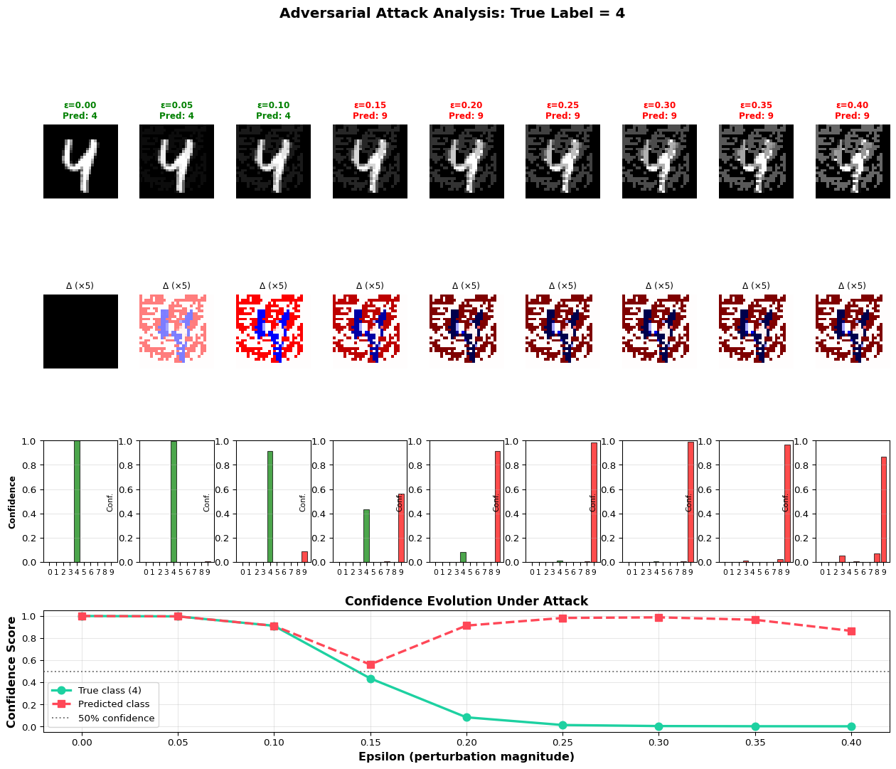
4. Perturbation Visualization
Visualize how adversarial perturbations affect model decisions:
Code
import numpy as npimport matplotlib.pyplot as pltfrom matplotlib.colors import LinearSegmentedColormap# Load pre-trained model and test image(x_train, y_train), (x_test, y_test) = tf.keras.datasets.mnist.load_data()x_test_norm = x_test.reshape(-1, 28, 28, 1) /255.0# Select test imagetest_idx =42original = x_test_norm[test_idx:test_idx+1]true_label = y_test[test_idx]print(f"=== Adversarial Perturbation Analysis ===")print(f"Original image label: {true_label}\n")# Generate perturbations with increasing epsilonepsilon_values = np.linspace(0, 0.4, 9)adversarial_examples = []predictions = []confidence_scores = []for eps in epsilon_values:if eps ==0: adv = originalelse: adv = fgsm_attack(model, original, true_label, eps) adversarial_examples.append(adv[0]) pred = model.predict(adv, verbose=0) pred_class = np.argmax(pred[0]) confidence = pred[0][pred_class] predictions.append(pred_class) confidence_scores.append(confidence)# Create comprehensive visualizationfig = plt.figure(figsize=(16, 12))gs = fig.add_gridspec(4, len(epsilon_values), hspace=0.4, wspace=0.3)# Row 1: Adversarial imagesfor i, (eps, adv, pred) inenumerate(zip(epsilon_values, adversarial_examples, predictions)): ax = fig.add_subplot(gs[0, i]) ax.imshow(adv.squeeze(), cmap='gray', vmin=0, vmax=1) color ='green'if pred == true_label else'red' ax.set_title(f'ε={eps:.2f}\nPred: {pred}', fontsize=9, color=color, fontweight='bold') ax.axis('off')# Row 2: Perturbations (amplified)for i, eps inenumerate(epsilon_values): ax = fig.add_subplot(gs[1, i])if eps >0: perturbation = adversarial_examples[i] - adversarial_examples[0] ax.imshow(perturbation.squeeze() *5, cmap='seismic', vmin=-1, vmax=1)else: ax.imshow(np.zeros_like(adversarial_examples[0].squeeze()), cmap='gray') ax.set_title(f'Δ (×5)', fontsize=9) ax.axis('off')# Row 3: Confidence heatmap for all classesfor i, eps inenumerate(epsilon_values): ax = fig.add_subplot(gs[2, i]) adv = adversarial_examples[i].reshape(1, 28, 28, 1) confidences = model.predict(adv, verbose=0)[0] colors = ['red'if j != true_label else'green'for j inrange(10)] bars = ax.bar(range(10), confidences, color=colors, alpha=0.7, edgecolor='black', linewidth=0.8) ax.set_ylim(0, 1) ax.set_xticks(range(10)) ax.set_xticklabels(range(10), fontsize=8) ax.set_ylabel('Conf.', fontsize=8) ax.grid(axis='y', alpha=0.3)if i ==0: ax.set_ylabel('Confidence', fontsize=9, fontweight='bold')# Row 4: Confidence evolution for true class and predicted classax_conf = fig.add_subplot(gs[3, :])true_class_conf = [model.predict(adv.reshape(1, 28, 28, 1), verbose=0)[0][true_label]for adv in adversarial_examples]predicted_class_conf = [model.predict(adv.reshape(1, 28, 28, 1), verbose=0)[0][pred]for adv, pred inzip(adversarial_examples, predictions)]ax_conf.plot(epsilon_values, true_class_conf, marker='o', linewidth=2.5, markersize=8, label=f'True class ({true_label})', color='#1dd1a1')ax_conf.plot(epsilon_values, predicted_class_conf, marker='s', linewidth=2.5, markersize=8, label='Predicted class', color='#ff4757', linestyle='--')ax_conf.axhline(y=0.5, color='gray', linestyle=':', label='50% confidence')ax_conf.set_xlabel('Epsilon (perturbation magnitude)', fontsize=12, fontweight='bold')ax_conf.set_ylabel('Confidence Score', fontsize=12, fontweight='bold')ax_conf.set_title('Confidence Evolution Under Attack', fontsize=13, fontweight='bold')ax_conf.legend(fontsize=10)ax_conf.grid(alpha=0.3)plt.suptitle(f'Adversarial Attack Analysis: True Label = {true_label}', fontsize=15, fontweight='bold', y=0.995)plt.show()# Statistical analysisprint("\n=== Attack Statistics ===")attack_success =sum([1for pred in predictions if pred != true_label])print(f"Attack success rate: {attack_success}/{len(predictions)} ({attack_success/len(predictions)*100:.1f}%)")print(f"Epsilon threshold for successful attack: {epsilon_values[predictions.index(next(p for p in predictions if p != true_label))]:.3f}")print(f"\nConfidence drop: {true_class_conf[0]:.3f} → {true_class_conf[-1]:.3f}")print(f"Most confused class: {predictions[-1]} (confidence: {confidence_scores[-1]:.3f})")print("\nInsight: Small perturbations (ε=0.1-0.2) can flip predictions while remaining imperceptible.")print("Defense strategies: adversarial training, input smoothing, ensemble methods.")
=== Adversarial Perturbation Analysis ===
Original image label: 4


=== Attack Statistics ===
Attack success rate: 6/9 (66.7%)
Epsilon threshold for successful attack: 0.150

Confidence drop: 1.000 → 0.001
Most confused class: 9 (confidence: 0.865)

Insight: Small perturbations (ε=0.1-0.2) can flip predictions while remaining imperceptible.
Defense strategies: adversarial training, input smoothing, ensemble methods.
Interactive Notebook
The notebook below contains runnable code for all Level 1 activities.
For edge devices, typical rate limits: - Sensor readings: 1-10 Hz - Image inference: 1-5 FPS - API queries: 10-100 per minute
Section 3: Adversarial Attack Demonstration
Adversarial examples are inputs designed to fool ML models while looking normal to humans.
📚 Theory: Adversarial Machine Learning
What Are Adversarial Examples?
An adversarial example is a modified input that: 1. Looks identical (or nearly identical) to the original to humans 2. Causes the model to make a confident wrong prediction
\(x_{adv} = x + \eta = x + \epsilon \cdot \text{sign}\left(\nabla_x J(\theta, x, y_{true})\right)\)
Where: - \(\nabla_x J\) = gradient of loss with respect to input - \(\text{sign}(\cdot)\) = element-wise sign function (+1, 0, or -1) - \(\epsilon\) = perturbation magnitude (controls visibility vs. effectiveness)
Why FGSM Works
Neural networks are locally linear in high-dimensional spaces:
\(w^T x_{adv} = w^T x + \epsilon \cdot w^T \text{sign}(w)\)
For a weight vector \(w\) with \(n\) dimensions and average magnitude \(m\):
\(\Delta = \epsilon \cdot m \cdot n\)
The activation change grows linearly with dimensionality. A 28×28 image has 784 dimensions, so even tiny \(\epsilon\) causes large activation changes!
Attack Strength vs. Visibility Trade-off
Epsilon (ε)
Perturbation
Attack Success
Human Visibility
0.01
Very small
Low (~20%)
Invisible
0.1
Small
Medium (~60%)
Barely visible
0.3
Large
High (~95%)
Visible if you look closely
📚 Understanding the Perturbation
L-infinity Norm Constraint
FGSM uses the L-infinity (L∞) norm to bound the perturbation:
For images with pixel values [0, 1]: - ε = 0.01: ~1/100th of dynamic range (imperceptible) - ε = 0.1: ~1/10th of dynamic range (barely visible) - ε = 0.3: ~1/3rd of dynamic range (noticeable)
Adversarial perturbations are typically: 1. High-frequency: Rapid pixel-to-pixel changes 2. Small magnitude: Near the noise floor 3. Precisely tuned: Specific to the exact pixel values
---title: "LAB06: Edge Security"subtitle: "Protecting ML Models and Data"---::: {.callout-note}## PDF Textbook ReferenceFor detailed theoretical foundations, mathematical proofs, and algorithm derivations, see **Chapter 6: Edge Security and Model Protection** in the [PDF textbook](../downloads/Edge-Analytics-Lab-Book-v1.0.0.pdf).The PDF chapter includes:- Comprehensive threat modeling frameworks for edge AI- Detailed analysis of adversarial attack techniques- Cryptographic foundations for model protection- Mathematical formulations of security-performance trade-offs- In-depth coverage of secure communication protocols:::[](https://colab.research.google.com/github/ngcharithperera/edge-analytics-lab-book/blob/main/notebooks/LAB06_edge_security.ipynb)[Download Notebook](https://raw.githubusercontent.com/ngcharithperera/edge-analytics-lab-book/main/notebooks/LAB06_edge_security.ipynb)## Learning ObjectivesBy the end of this lab you will be able to:- Describe the main attack surfaces of an edge ML device- Construct a simple threat model for an edge AI application- Implement basic input validation and sanity checks- Understand how adversarial examples are generated and why they work- Apply simple model protection techniques (checksums, obfuscation, encrypted storage) on constrained devices## Theory Summary### Security Challenges for Edge ML SystemsEdge devices face unique security challenges that cloud systems never encounter - they exist in the physical world where attackers can touch, probe, and manipulate them. Understanding these threats and implementing practical defenses is essential for robust edge ML deployment.**Why Edge Devices Are Vulnerable:** Unlike cloud servers protected in secure data centers, edge devices are exposed. An attacker with physical access can extract firmware via JTAG/SWD, dump Flash memory to steal your trained model, intercept network traffic, feed malicious sensor inputs, or even replace components. Your $15 Arduino sitting on a desk is fundamentally harder to protect than a server rack behind locked doors with armed guards.**The Four Attack Surfaces:** Edge ML devices have four main vulnerability points: (1) Network attacks via WiFi/BLE (eavesdropping, command injection), (2) Physical access (firmware extraction, hardware tampering), (3) Malicious inputs (adversarial examples, sensor spoofing), and (4) Model extraction (stealing your trained intellectual property). Each requires different defensive strategies, and perfect security is impossible - we aim for "good enough" security proportional to the application's risk.**Input Validation - The First Line of Defense:** Before feeding data to your model, validate it: check data types (is it a numpy array?), shapes (28×28 pixels?), value ranges (0-255?), and detect NaN/Inf. This prevents crashes from malformed inputs and catches many attacks. On microcontrollers, add bounds checks, sanitize sensor readings, and use timeout watchdogs. Simple validation stops 80% of attacks with 20% effort.**Adversarial Examples - Fooling ML Models:** Adversarial examples are inputs crafted to fool neural networks - images with imperceptible noise that flip predictions from "stop sign" to "speed limit." They work because neural networks learn decision boundaries in high-dimensional space, and adversarial perturbations push inputs across these boundaries. Defense strategies include input smoothing, adversarial training (include adversarial examples in training data), and ensemble methods. No perfect defense exists, but we can make attacks harder.**Model Protection Strategies:** To protect your trained model from extraction: (1) Add checksums or HMAC to detect tampering, (2) Encrypt the .tflite file and decrypt at runtime (careful - keys must be stored somewhere!), (3) Use hardware security modules (HSM) like ATECC608 on production devices, (4) Obfuscate model architecture (limited effectiveness), (5) Use secure boot to prevent firmware modification. Remember: if an attacker has physical access and unlimited time, they can extract anything - we just make it expensive enough to deter most attackers.## Key Concepts at a Glance::: {.callout-note icon=false}## Core Concepts- **Attack Surface**: Points where an attacker can interact with or compromise a system- **Threat Model**: Structured analysis of potential threats, attackers, and impacts- **Input Validation**: Checking inputs before processing to prevent crashes and attacks- **Adversarial Examples**: Maliciously crafted inputs that fool ML models- **FGSM**: Fast Gradient Sign Method - simple adversarial attack technique- **Model Extraction**: Stealing trained models via firmware dumps or API queries- **Secure Boot**: Cryptographic verification of firmware integrity at startup- **HMAC**: Hash-based Message Authentication Code for integrity checking:::## Common Pitfalls::: {.callout-warning}## Mistakes to Avoid**Hardcoding Credentials in Firmware**: Never put WiFi passwords, API keys, or encryption keys directly in source code! Once firmware is uploaded to a device, anyone with physical access can extract these secrets using simple tools (esptool, OpenOCD). Instead: store credentials in separate config files excluded from version control, use secure elements when available, or implement secure provisioning processes.**Trusting Sensor Inputs Blindly**: Sensors can fail, be spoofed, or send garbage data. A temperature sensor might report -273°C (impossible), an accelerometer might saturate at max values (stuck or vibrating), or an attacker might inject false readings. Always validate: check plausible ranges, detect impossible transitions, use median filtering, and implement timeout watchdogs.**Ignoring Side-Channel Attacks**: Power analysis attacks can extract encryption keys by measuring tiny variations in power consumption during crypto operations. Timing attacks infer internal state by measuring how long operations take. On high-security applications (payment, authentication), use constant-time algorithms and hardware crypto modules that resist these attacks.**Security Theater vs Real Security**: Adding a simple XOR "encryption" or hex encoding doesn't provide security - it just makes code harder to read. Real security requires: proper cryptography (AES, not ROT13), secure key management (not hardcoded), threat modeling (know your attackers), and defense in depth (multiple layers). Don't confuse obscurity with security.**Over-Engineering Security for Low-Risk Applications**: A hobby weather station doesn't need military-grade encryption. Security has costs: code complexity, CPU cycles, development time, and power consumption. Match security level to actual risk. For a smart light bulb, basic input validation is fine. For a medical device or industrial controller, invest in proper security.:::## Quick Reference### Key Formulas**Adversarial Perturbation (FGSM):**$$x_{adv} = x + \epsilon \cdot \text{sign}(\nabla_x L(\theta, x, y))$$where $\epsilon$ controls perturbation magnitude (typically 0.01-0.3)**HMAC for Model Integrity:**$$\text{HMAC}(K, M) = H((K \oplus \text{opad}) \| H((K \oplus \text{ipad}) \| M))$$Verify: compute HMAC of model data, compare with stored hash**AES Encryption Overhead:**$$\text{Encrypted Size} = \text{Original Size} + 16 \text{ bytes (IV)}$$**Security Level Estimation:**$$\text{Bits of Security} \approx \log_2(\text{Key Space})$$128-bit key = $2^{128}$ possible keys (effectively unbreakable)### Important Parameter Values**Attack Difficulty Levels:**| Attacker Type | Access | Cost | Mitigation ||---------------|--------|------|------------|| Remote (Internet) | Network only | Low | Firewall, TLS, rate limiting || Local (Same network) | WiFi/BLE range | Medium | Authentication, encryption || Physical (Device access) | Can touch device | High | Secure boot, tamper detection || Lab (Unlimited time) | Full equipment | Very High | Accept some risk unavoidable |**Common Security Measures:**| Technique | Complexity | Effectiveness | Use Case ||-----------|------------|---------------|----------|| Input validation | Low | High | Always implement || HTTPS/TLS | Medium | High | Network communication || AES encryption | Medium | High | Sensitive data storage || Secure boot | High | Very High | Production devices || Hardware HSM | High | Very High | High-security applications |**Code Patterns:**```python# Python input validationdef validate_input(data, expected_shape, value_range):ifnotisinstance(data, np.ndarray):returnFalse, "Not numpy array"if data.shape != expected_shape:returnFalse, f"Wrong shape: {data.shape}"if data.min() < value_range[0] or data.max() > value_range[1]:returnFalse, "Values out of range"if np.isnan(data).any() or np.isinf(data).any():returnFalse, "Contains NaN/Inf"returnTrue, "Valid"``````cpp// Arduino bounds checkingbool validateSensorReading(float value,float min_val,float max_val){if(isnan(value)|| isinf(value))returnfalse;if(value < min_val || value > max_val)returnfalse;returntrue;}```### Links to PDF SectionsFor deeper understanding, see these sections in [Chapter 6 PDF](../downloads/Edge-Analytics-Lab-Book-v1.0.0.pdf#page=131):- **Section 6.1**: Why Security Matters for Edge AI (pages 132-135)- **Section 6.2**: Building a Threat Model (pages 136-139)- **Section 6.3**: Input Validation (pages 140-144)- **Section 6.4**: Adversarial Examples (pages 145-151)- **Section 6.5**: Model Protection Techniques (pages 152-157)- **Section 6.6**: Secure Communication (pages 158-162)- **Exercises**: Secure your edge ML system (pages 163-164)### Interactive Learning Tools::: {.callout-tip}## Explore Security ConceptsUnderstand attacks and defenses interactively:- **[TensorFlow FGSM Tutorial](https://colab.research.google.com/github/tensorflow/docs/blob/master/site/en/tutorials/generative/adversarial_fgsm.ipynb)** - Generate adversarial examples step-by-step and see how tiny perturbations fool classifiers- **[Our Adversarial Attack Demo](../simulations/adversarial-attack.qmd)** - Visualize FGSM attacks on MNIST and experiment with different epsilon values- **[Threat Modeling Worksheet](../simulations/threat-model-template.qmd)** - Interactive template for building threat models for your edge ML application:::## Self-Assessment CheckpointsTest your understanding before proceeding to the exercises.::: {.callout-note collapse="true" title="Question 1: List the four main attack surfaces for edge ML devices and give an example attack for each."}**Answer:** (1) **Network**: WiFi/BLE eavesdropping to capture sensitive data, command injection via unvalidated API calls, (2) **Physical access**: Firmware extraction via JTAG/SWD to steal models, replacing sensor with malicious inputs, (3) **Malicious inputs**: Adversarial examples to fool classifiers, sensor spoofing (fake GPS, temperature), (4) **Model extraction**: Stealing trained models via memory dumps or API queries to replicate proprietary ML. Each requires different defenses: network (TLS, authentication), physical (secure boot, tamper detection), inputs (validation, adversarial training), model (encryption, obfuscation).:::::: {.callout-note collapse="true" title="Question 2: Calculate the adversarial perturbation for an input pixel value of 0.8 with epsilon=0.1 and gradient sign = +1."}**Answer:** Using FGSM formula: x_adv = x + ε × sign(gradient) = 0.8 + 0.1 × (+1) = 0.8 + 0.1 = 0.9. The adversarial pixel value is 0.9 (assuming we clip to valid range 0-1). This tiny perturbation (0.1 difference) is often imperceptible to humans but can flip a classifier's prediction. If the gradient sign were -1, the result would be 0.8 - 0.1 = 0.7. Epsilon controls attack strength: larger ε = more visible perturbation but stronger attack.:::::: {.callout-note collapse="true" title="Question 3: You stored your WiFi password directly in Arduino code: `const char* password = 'MySecret123';`. Why is this a security problem?"}**Answer:** Once you upload firmware to a device, anyone with physical access can extract it using simple tools (esptool for ESP32, OpenOCD for ARM). They'll get the complete binary including your hardcoded password in plain text. Solutions: (1) Store credentials in separate config files excluded from version control, (2) Use secure elements (ATECC608) to store secrets in hardware, (3) Implement secure provisioning where users enter credentials via app/web interface instead of hardcoding, (4) For development, use environment variables. Never commit secrets to GitHub - once they're in git history, they're public forever.:::::: {.callout-note collapse="true" title="Question 4: Your temperature sensor occasionally reports -273°C. Should your system accept this reading?"}**Answer:** No! -273°C is absolute zero (physically impossible in normal conditions). This indicates sensor failure, loose wiring, or malicious input. Always validate: `if (temp < -40 || temp > 85) { /* reject */ }` for typical environments. Additional checks: detect impossible transitions (10°C to 100°C in 1 second), use median filtering to reject outliers, implement timeout watchdogs, and cross-validate with multiple sensors when critical. Accepting invalid sensor data causes: crashes (division by zero), incorrect decisions (false alarms), or security vulnerabilities (bypassing safety limits).:::::: {.callout-note collapse="true" title="Question 5: When is investing in hardware security modules (HSM) like ATECC608 justified vs overkill?"}**Answer:** **Use HSM for**: Payment systems (credit cards), authentication tokens (2FA devices), medical devices (regulatory requirements), industrial control (safety-critical), any device handling cryptographic keys for more than test purposes. **HSM is overkill for**: Hobby projects, smart home lights, weather stations, non-critical sensors, prototypes. HSMs add cost ($1-5 per device), complexity (new APIs to learn), and development time. Match security to risk: a $5 smart bulb doesn't need military-grade encryption, but a $500 insulin pump absolutely does. Use threat modeling to decide.:::## Try It Yourself: Executable Python ExamplesThe following code blocks demonstrate security concepts for edge ML systems. These examples are fully executable and include visualizations.### 1. FGSM Adversarial Attack DemoGenerate adversarial examples using the Fast Gradient Sign Method:```{python}import tensorflow as tfimport numpy as npimport matplotlib.pyplot as plt# Load MNIST datasetprint("=== Loading MNIST Dataset ===")(x_train, y_train), (x_test, y_test) = tf.keras.datasets.mnist.load_data()x_test = x_test /255.0# Normalize to [0, 1]x_test = x_test.reshape(-1, 28, 28, 1).astype(np.float32)# Train a simple CNNprint("Training classifier...")model = tf.keras.Sequential([ tf.keras.layers.Conv2D(32, (3, 3), activation='relu', input_shape=(28, 28, 1)), tf.keras.layers.MaxPooling2D((2, 2)), tf.keras.layers.Conv2D(64, (3, 3), activation='relu'), tf.keras.layers.MaxPooling2D((2, 2)), tf.keras.layers.Flatten(), tf.keras.layers.Dense(128, activation='relu'), tf.keras.layers.Dense(10, activation='softmax')])model.compile(optimizer='adam', loss='sparse_categorical_crossentropy', metrics=['accuracy'])x_train_norm = x_train.reshape(-1, 28, 28, 1) /255.0model.fit(x_train_norm, y_train, epochs=3, batch_size=128, verbose=0, validation_split=0.1)# Evaluate on clean test settest_loss, test_acc = model.evaluate(x_test, y_test, verbose=0)print(f"\nClean test accuracy: {test_acc*100:.2f}%")# FGSM attack implementationdef fgsm_attack(model, image, label, epsilon):""" Generate adversarial example using Fast Gradient Sign Method. Args: model: Trained classifier image: Input image (28x28x1) label: True label epsilon: Perturbation magnitude (typically 0.01-0.3) """ image = tf.convert_to_tensor(image, dtype=tf.float32) label = tf.convert_to_tensor([label], dtype=tf.int64)with tf.GradientTape() as tape: tape.watch(image) prediction = model(image) loss = tf.keras.losses.sparse_categorical_crossentropy(label, prediction)# Get gradient of loss with respect to image gradient = tape.gradient(loss, image)# Create adversarial image: x_adv = x + epsilon * sign(gradient) signed_grad = tf.sign(gradient) adversarial_image = image + epsilon * signed_grad# Clip to valid range [0, 1] adversarial_image = tf.clip_by_value(adversarial_image, 0, 1)return adversarial_image.numpy()# Generate adversarial examples with different epsilon valuesprint("\n=== Generating Adversarial Examples ===")test_idx =0original_image = x_test[test_idx:test_idx+1]true_label = y_test[test_idx]epsilons = [0.0, 0.05, 0.1, 0.2, 0.3]adversarial_images = []predictions = []confidences = []for eps in epsilons:if eps ==0: adv_img = original_imageelse: adv_img = fgsm_attack(model, original_image, true_label, eps) adversarial_images.append(adv_img[0])# Get prediction pred = model.predict(adv_img, verbose=0) pred_class = np.argmax(pred[0]) confidence = np.max(pred[0]) predictions.append(pred_class) confidences.append(confidence)print(f"ε={eps:.2f}: Predicted={pred_class} (confidence={confidence:.3f}) | True={true_label}")# Visualize adversarial examplesfig, axes = plt.subplots(2, len(epsilons), figsize=(15, 6))for i, (eps, adv_img, pred, conf) inenumerate(zip(epsilons, adversarial_images, predictions, confidences)):# Original/adversarial image axes[0, i].imshow(adv_img.squeeze(), cmap='gray', vmin=0, vmax=1) axes[0, i].set_title(f'ε={eps:.2f}', fontsize=11, fontweight='bold') axes[0, i].axis('off')# Perturbation (amplified for visibility)if eps >0: perturbation = adv_img - adversarial_images[0] axes[1, i].imshow(perturbation.squeeze() *10, cmap='seismic', vmin=-1, vmax=1)else: axes[1, i].imshow(np.zeros_like(adv_img.squeeze()), cmap='gray') color ='green'if pred == true_label else'red' axes[1, i].set_title(f'Pred: {pred} ({conf:.2f})', fontsize=10, color=color, fontweight='bold') axes[1, i].axis('off')axes[0, 0].set_ylabel('Adversarial\nImage', fontsize=12, fontweight='bold')axes[1, 0].set_ylabel('Perturbation\n(×10)', fontsize=12, fontweight='bold')plt.suptitle(f'FGSM Attack on MNIST (True Label: {true_label})', fontsize=14, fontweight='bold')plt.tight_layout()plt.show()# Calculate attack success rate across multiple samplesprint("\n=== Attack Success Rate Across Test Set ===")num_samples =100success_rates = []for eps in [0.0, 0.05, 0.1, 0.15, 0.2, 0.25, 0.3]: correct =0for i inrange(num_samples): img = x_test[i:i+1] label = y_test[i]if eps ==0: adv_img = imgelse: adv_img = fgsm_attack(model, img, label, eps) pred = model.predict(adv_img, verbose=0)if np.argmax(pred[0]) == label: correct +=1 accuracy = correct / num_samples success_rates.append(accuracy)print(f"ε={eps:.2f}: Accuracy = {accuracy*100:.1f}% (attack success = {(1-accuracy)*100:.1f}%)")# Plot accuracy vs epsilonplt.figure(figsize=(10, 6))eps_values = [0.0, 0.05, 0.1, 0.15, 0.2, 0.25, 0.3]plt.plot(eps_values, [s*100for s in success_rates], marker='o', linewidth=2, markersize=8, color='#ff6b6b')plt.axhline(y=50, color='gray', linestyle='--', label='Random guess (10 classes)')plt.xlabel('Epsilon (perturbation magnitude)', fontsize=12, fontweight='bold')plt.ylabel('Model Accuracy (%)', fontsize=12, fontweight='bold')plt.title('FGSM Attack Effectiveness vs Perturbation Magnitude', fontsize=14, fontweight='bold')plt.grid(alpha=0.3)plt.legend()plt.tight_layout()plt.show()print("\nInsight: Adversarial attacks can fool neural networks with imperceptible perturbations.")print("Even small epsilon values (0.1-0.2) significantly reduce accuracy from ~99% to <60%.")```### 2. Input Validation ImplementationDemonstrate comprehensive input validation for edge ML systems:```{python}import numpy as npimport matplotlib.pyplot as pltimport pandas as pddef validate_input(data, expected_shape, value_range, dtype_expected=np.float32):""" Comprehensive input validation for ML models. Args: data: Input data to validate expected_shape: Tuple of expected dimensions value_range: Tuple of (min, max) valid values dtype_expected: Expected numpy data type Returns: (is_valid, error_message) """ validations = []# Check 1: Is it a numpy array?ifnotisinstance(data, np.ndarray):returnFalse, "Not a numpy array", validations validations.append(("Type check", True, "numpy.ndarray"))# Check 2: Correct shape? shape_match = data.shape == expected_shape validations.append(("Shape check", shape_match,f"Expected {expected_shape}, got {data.shape}"))ifnot shape_match:returnFalse, f"Shape mismatch: expected {expected_shape}, got {data.shape}", validations# Check 3: Correct data type? dtype_match = data.dtype == dtype_expected validations.append(("Data type", dtype_match,f"Expected {dtype_expected}, got {data.dtype}"))# Check 4: Value range min_val, max_val = value_range values_in_range = (data.min() >= min_val) and (data.max() <= max_val) validations.append(("Value range", values_in_range,f"Min={data.min():.3f}, Max={data.max():.3f}, Expected [{min_val}, {max_val}]"))ifnot values_in_range:returnFalse, f"Values out of range: [{data.min():.3f}, {data.max():.3f}] not in [{min_val}, {max_val}]", validations# Check 5: No NaN or Inf has_invalid = np.isnan(data).any() or np.isinf(data).any() validations.append(("NaN/Inf check", not has_invalid,f"Contains NaN: {np.isnan(data).any()}, Contains Inf: {np.isinf(data).any()}"))if has_invalid:returnFalse, "Contains NaN or Inf values", validations# Check 6: Not all zeros (suspicious) all_zeros = np.all(data ==0) validations.append(("Non-zero data", not all_zeros,f"All zeros: {all_zeros}"))if all_zeros:returnFalse, "Warning: All values are zero (sensor failure?)", validationsreturnTrue, "All validations passed", validations# Test with various input scenariosprint("=== Input Validation Test Suite ===\n")test_cases = [ ("Valid input", np.random.rand(28, 28).astype(np.float32), (28, 28), (0, 1), np.float32), ("Wrong shape", np.random.rand(32, 32).astype(np.float32), (28, 28), (0, 1), np.float32), ("Values out of range", np.random.rand(28, 28).astype(np.float32) *2, (28, 28), (0, 1), np.float32), ("Contains NaN", np.full((28, 28), np.nan, dtype=np.float32), (28, 28), (0, 1), np.float32), ("Contains Inf", np.full((28, 28), np.inf, dtype=np.float32), (28, 28), (0, 1), np.float32), ("All zeros", np.zeros((28, 28), dtype=np.float32), (28, 28), (0, 1), np.float32), ("Wrong dtype", np.random.randint(0, 255, (28, 28), dtype=np.uint8), (28, 28), (0, 1), np.float32),]results = []for name, data, shape, val_range, dtype in test_cases: is_valid, message, checks = validate_input(data, shape, val_range, dtype) results.append({'Test Case': name,'Valid': '✓'if is_valid else'✗','Message': message })print(f"Test: {name}")print(f" Result: {'PASS'if is_valid else'FAIL'}")print(f" Message: {message}\n")# Summary tabledf_results = pd.DataFrame(results)print("=== Validation Summary ===")print(df_results.to_string(index=False))# Visualize validation checks for one test caseprint("\n=== Detailed Validation Breakdown: Valid Input ===")valid_data = np.random.rand(28, 28).astype(np.float32)is_valid, message, checks = validate_input(valid_data, (28, 28), (0, 1), np.float32)check_names = [c[0] for c in checks]check_results = [c[1] for c in checks]check_details = [c[2] for c in checks]fig, (ax1, ax2) = plt.subplots(1, 2, figsize=(14, 5))# Bar chart of validation checkscolors = ['#1dd1a1'if result else'#ff4757'for result in check_results]bars = ax1.barh(check_names, [1]*len(check_names), color=colors, edgecolor='black', linewidth=1.5)ax1.set_xlim(0, 1)ax1.set_xlabel('Status', fontsize=11)ax1.set_title('Input Validation Checks', fontsize=13, fontweight='bold')ax1.set_xticks([])# Add labelsfor i, (bar, result) inenumerate(zip(bars, check_results)): label ='✓ PASS'if result else'✗ FAIL' ax1.text(0.5, bar.get_y() + bar.get_height()/2, label, ha='center', va='center', fontweight='bold', fontsize=11, color='white')# Image of validated inputax2.imshow(valid_data, cmap='viridis')ax2.set_title(f'Validated Input Image\n{valid_data.shape}', fontsize=13, fontweight='bold')ax2.axis('off')plt.tight_layout()plt.show()print("\nInsight: Input validation prevents crashes, detects sensor failures, and catches malicious inputs.")print("Always validate: data type, shape, value range, and check for NaN/Inf before inference.")```### 3. Simple Encryption/Decryption ExampleDemonstrate model protection using AES encryption:```{python}import numpy as npimport matplotlib.pyplot as pltfrom cryptography.hazmat.primitives.ciphers import Cipher, algorithms, modesfrom cryptography.hazmat.backends import default_backendimport osimport timedef encrypt_model(model_data, key):""" Encrypt model data using AES-256 encryption. Args: model_data: Bytes of model file key: 32-byte encryption key Returns: (iv, encrypted_data) tuple """# Generate random initialization vector (IV) iv = os.urandom(16)# Create cipher cipher = Cipher( algorithms.AES(key), modes.CBC(iv), backend=default_backend() ) encryptor = cipher.encryptor()# Pad data to multiple of 16 bytes (AES block size) padding_length =16- (len(model_data) %16) padded_data = model_data +bytes([padding_length] * padding_length)# Encrypt encrypted_data = encryptor.update(padded_data) + encryptor.finalize()return iv, encrypted_datadef decrypt_model(iv, encrypted_data, key):""" Decrypt model data using AES-256. Args: iv: Initialization vector (16 bytes) encrypted_data: Encrypted model bytes key: 32-byte encryption key Returns: Decrypted model data """ cipher = Cipher( algorithms.AES(key), modes.CBC(iv), backend=default_backend() ) decryptor = cipher.decryptor() decrypted_padded = decryptor.update(encrypted_data) + decryptor.finalize()# Remove padding padding_length = decrypted_padded[-1] decrypted_data = decrypted_padded[:-padding_length]return decrypted_data# Simulate model data (random bytes representing a .tflite model)print("=== Model Encryption Demo ===\n")model_size_kb =50model_data = os.urandom(model_size_kb *1024) # 50 KB modelprint(f"Original model size: {len(model_data) /1024:.1f} KB")# Generate encryption key (in production, use secure key management!)encryption_key = os.urandom(32) # 256-bit keyprint(f"Encryption key: {encryption_key.hex()[:32]}... (256 bits)")# Encrypt modelstart_time = time.perf_counter()iv, encrypted_model = encrypt_model(model_data, encryption_key)encryption_time = (time.perf_counter() - start_time) *1000print(f"\nEncryption time: {encryption_time:.2f} ms")print(f"Encrypted size: {len(encrypted_model) /1024:.1f} KB (+ 16 bytes IV)")print(f"IV: {iv.hex()}")# Decrypt modelstart_time = time.perf_counter()decrypted_model = decrypt_model(iv, encrypted_model, encryption_key)decryption_time = (time.perf_counter() - start_time) *1000print(f"\nDecryption time: {decryption_time:.2f} ms")print(f"Decrypted size: {len(decrypted_model) /1024:.1f} KB")# Verify decryptionis_correct = model_data == decrypted_modelprint(f"\nDecryption successful: {is_correct}")# Visualize encryption processfig, axes = plt.subplots(2, 2, figsize=(14, 10))# Original model data (first 1024 bytes visualized as 32x32 grid)original_grid = np.frombuffer(model_data[:1024], dtype=np.uint8).reshape(32, 32)axes[0, 0].imshow(original_grid, cmap='viridis')axes[0, 0].set_title('Original Model Data\n(First 1024 bytes)', fontsize=12, fontweight='bold')axes[0, 0].axis('off')# Encrypted model dataencrypted_grid = np.frombuffer(encrypted_model[:1024], dtype=np.uint8).reshape(32, 32)axes[0, 1].imshow(encrypted_grid, cmap='plasma')axes[0, 1].set_title('Encrypted Model Data\n(First 1024 bytes)', fontsize=12, fontweight='bold')axes[0, 1].axis('off')# Decrypted model datadecrypted_grid = np.frombuffer(decrypted_model[:1024], dtype=np.uint8).reshape(32, 32)axes[1, 0].imshow(decrypted_grid, cmap='viridis')axes[1, 0].set_title('Decrypted Model Data\n(Matches original)', fontsize=12, fontweight='bold')axes[1, 0].axis('off')# Byte distribution comparisonaxes[1, 1].hist(np.frombuffer(model_data, dtype=np.uint8), bins=50, alpha=0.6, label='Original', color='#4ecdc4', edgecolor='black')axes[1, 1].hist(np.frombuffer(encrypted_model, dtype=np.uint8), bins=50, alpha=0.6, label='Encrypted', color='#ff6b6b', edgecolor='black')axes[1, 1].set_xlabel('Byte Value', fontsize=11)axes[1, 1].set_ylabel('Frequency', fontsize=11)axes[1, 1].set_title('Byte Distribution Comparison', fontsize=12, fontweight='bold')axes[1, 1].legend()axes[1, 1].grid(alpha=0.3)plt.tight_layout()plt.show()# Performance analysisprint("\n=== Performance Analysis ===")model_sizes = [10, 25, 50, 100, 200, 500] # KBenc_times = []dec_times = []for size_kb in model_sizes: data = os.urandom(size_kb *1024)# Encryption start = time.perf_counter() iv, enc = encrypt_model(data, encryption_key) enc_times.append((time.perf_counter() - start) *1000)# Decryption start = time.perf_counter() dec = decrypt_model(iv, enc, encryption_key) dec_times.append((time.perf_counter() - start) *1000)# Plot performanceplt.figure(figsize=(10, 6))plt.plot(model_sizes, enc_times, marker='o', linewidth=2, markersize=8, label='Encryption', color='#ff6b6b')plt.plot(model_sizes, dec_times, marker='s', linewidth=2, markersize=8, label='Decryption', color='#45b7d1')plt.xlabel('Model Size (KB)', fontsize=12, fontweight='bold')plt.ylabel('Time (ms)', fontsize=12, fontweight='bold')plt.title('AES-256 Encryption/Decryption Performance', fontsize=14, fontweight='bold')plt.legend(fontsize=11)plt.grid(alpha=0.3)plt.tight_layout()plt.show()print("\nInsight: AES-256 encryption protects models from extraction but adds runtime overhead.")print(f"For a {model_size_kb} KB model: encrypt={encryption_time:.1f}ms, decrypt={decryption_time:.1f}ms")print("Trade-off: Security (prevents firmware dumps) vs Performance (decryption cost at startup).")```### 4. Perturbation VisualizationVisualize how adversarial perturbations affect model decisions:```{python}import numpy as npimport matplotlib.pyplot as pltfrom matplotlib.colors import LinearSegmentedColormap# Load pre-trained model and test image(x_train, y_train), (x_test, y_test) = tf.keras.datasets.mnist.load_data()x_test_norm = x_test.reshape(-1, 28, 28, 1) /255.0# Select test imagetest_idx =42original = x_test_norm[test_idx:test_idx+1]true_label = y_test[test_idx]print(f"=== Adversarial Perturbation Analysis ===")print(f"Original image label: {true_label}\n")# Generate perturbations with increasing epsilonepsilon_values = np.linspace(0, 0.4, 9)adversarial_examples = []predictions = []confidence_scores = []for eps in epsilon_values:if eps ==0: adv = originalelse: adv = fgsm_attack(model, original, true_label, eps) adversarial_examples.append(adv[0]) pred = model.predict(adv, verbose=0) pred_class = np.argmax(pred[0]) confidence = pred[0][pred_class] predictions.append(pred_class) confidence_scores.append(confidence)# Create comprehensive visualizationfig = plt.figure(figsize=(16, 12))gs = fig.add_gridspec(4, len(epsilon_values), hspace=0.4, wspace=0.3)# Row 1: Adversarial imagesfor i, (eps, adv, pred) inenumerate(zip(epsilon_values, adversarial_examples, predictions)): ax = fig.add_subplot(gs[0, i]) ax.imshow(adv.squeeze(), cmap='gray', vmin=0, vmax=1) color ='green'if pred == true_label else'red' ax.set_title(f'ε={eps:.2f}\nPred: {pred}', fontsize=9, color=color, fontweight='bold') ax.axis('off')# Row 2: Perturbations (amplified)for i, eps inenumerate(epsilon_values): ax = fig.add_subplot(gs[1, i])if eps >0: perturbation = adversarial_examples[i] - adversarial_examples[0] ax.imshow(perturbation.squeeze() *5, cmap='seismic', vmin=-1, vmax=1)else: ax.imshow(np.zeros_like(adversarial_examples[0].squeeze()), cmap='gray') ax.set_title(f'Δ (×5)', fontsize=9) ax.axis('off')# Row 3: Confidence heatmap for all classesfor i, eps inenumerate(epsilon_values): ax = fig.add_subplot(gs[2, i]) adv = adversarial_examples[i].reshape(1, 28, 28, 1) confidences = model.predict(adv, verbose=0)[0] colors = ['red'if j != true_label else'green'for j inrange(10)] bars = ax.bar(range(10), confidences, color=colors, alpha=0.7, edgecolor='black', linewidth=0.8) ax.set_ylim(0, 1) ax.set_xticks(range(10)) ax.set_xticklabels(range(10), fontsize=8) ax.set_ylabel('Conf.', fontsize=8) ax.grid(axis='y', alpha=0.3)if i ==0: ax.set_ylabel('Confidence', fontsize=9, fontweight='bold')# Row 4: Confidence evolution for true class and predicted classax_conf = fig.add_subplot(gs[3, :])true_class_conf = [model.predict(adv.reshape(1, 28, 28, 1), verbose=0)[0][true_label]for adv in adversarial_examples]predicted_class_conf = [model.predict(adv.reshape(1, 28, 28, 1), verbose=0)[0][pred]for adv, pred inzip(adversarial_examples, predictions)]ax_conf.plot(epsilon_values, true_class_conf, marker='o', linewidth=2.5, markersize=8, label=f'True class ({true_label})', color='#1dd1a1')ax_conf.plot(epsilon_values, predicted_class_conf, marker='s', linewidth=2.5, markersize=8, label='Predicted class', color='#ff4757', linestyle='--')ax_conf.axhline(y=0.5, color='gray', linestyle=':', label='50% confidence')ax_conf.set_xlabel('Epsilon (perturbation magnitude)', fontsize=12, fontweight='bold')ax_conf.set_ylabel('Confidence Score', fontsize=12, fontweight='bold')ax_conf.set_title('Confidence Evolution Under Attack', fontsize=13, fontweight='bold')ax_conf.legend(fontsize=10)ax_conf.grid(alpha=0.3)plt.suptitle(f'Adversarial Attack Analysis: True Label = {true_label}', fontsize=15, fontweight='bold', y=0.995)plt.show()# Statistical analysisprint("\n=== Attack Statistics ===")attack_success =sum([1for pred in predictions if pred != true_label])print(f"Attack success rate: {attack_success}/{len(predictions)} ({attack_success/len(predictions)*100:.1f}%)")print(f"Epsilon threshold for successful attack: {epsilon_values[predictions.index(next(p for p in predictions if p != true_label))]:.3f}")print(f"\nConfidence drop: {true_class_conf[0]:.3f} → {true_class_conf[-1]:.3f}")print(f"Most confused class: {predictions[-1]} (confidence: {confidence_scores[-1]:.3f})")print("\nInsight: Small perturbations (ε=0.1-0.2) can flip predictions while remaining imperceptible.")print("Defense strategies: adversarial training, input smoothing, ensemble methods.")```## Interactive NotebookThe notebook below contains runnable code for all Level 1 activities.{{< embed ../../notebooks/LAB06_edge_security.ipynb >}}## Three-Tier Activities::: {.panel-tabset}### Level 1: NotebookRun the embedded notebook above. Key exercises:1. Follow along with the code cells2. Modify parameters and observe results3. Complete the checkpoint questions### Level 2: SimulatorUse Level 2 to explore attacks and defenses without risking real devices:**[TensorFlow FGSM Tutorial](https://colab.research.google.com/github/tensorflow/docs/blob/master/site/en/tutorials/generative/adversarial_fgsm.ipynb)** – Interactive adversarial attack demo:- Generate adversarial examples step-by-step- See how small perturbations fool classifiers- Experiment with different epsilon values**[Our Adversarial Attack Demo](../simulations/adversarial-attack.qmd)** – Visualize FGSM attacks on MNIST and experiment with different threat scenarios### Level 3: DeviceOn-device, focus on \emph{simple, practical protections}:- Add a \textbf{model checksum} or version tag in firmware and verify it at boot- Implement basic \textbf{input validation} (e.g., range checks on sensor values)- Use HTTPS/TLS (on Pi) or pre-shared keys (on MCUs) for communication where feasibleIf you are working with earlier labs (KWS or CV), consider:1. Adding plausibility checks for sensor inputs (e.g., audio energy thresholds, image brightness). 2. Logging unexpected patterns for offline analysis. 3. Documenting which threats your design mitigates and which remain open.:::## Related Labs::: {.callout-tip}## Security & Privacy- **LAB17: Federated Learning** - Privacy-preserving distributed training- **LAB13: Distributed Data** - Secure data pipelines:::::: {.callout-tip}## Apply Security Concepts- **LAB04: Keyword Spotting** - Secure audio ML pipelines- **LAB07: CNNs & Vision** - Adversarial robustness for vision models- **LAB09: ESP32 Wireless** - Secure network communication:::## Related Resources- [Hardware Guide](../resources/hardware.qmd) - Equipment needed for Level 3- [Troubleshooting](../resources/troubleshooting.qmd) - Common issues and solutions