LAB16: YOLO Object Detection

Real-Time Computer Vision

PDF Textbook Reference

For detailed theoretical foundations, mathematical proofs, and algorithm derivations, see Chapter 16: Real-Time Computer Vision and Object Detection in the PDF textbook.

The PDF chapter includes: - Complete mathematical formulation of YOLO architecture - Detailed derivations of bounding box regression and IoU metrics - In-depth coverage of Non-Maximum Suppression (NMS) algorithms - Comprehensive analysis of anchor boxes and feature pyramids - Theoretical foundations for real-time vision system design

Open In Colab

Download Notebook

Learning Objectives

By the end of this lab you should be able to:

Explain the difference between one-stage and two-stage object detectors and why YOLO/Tiny-YOLO are preferred for edge
Interpret YOLO outputs (grids, anchors, confidences, NMS) on images and video
Measure and reason about FPS, latency, and model size for different YOLO variants on edge hardware
Deploy a Tiny-YOLO style model on Raspberry Pi and evaluate its suitability for a given application

Theory Summary

YOLO: You Only Look Once

Traditional object detection uses two stages: (1) generate region proposals (where objects might be), (2) classify each region. This is slow—unacceptable for real-time edge applications.

YOLO revolutionized object detection by treating it as a single regression problem: one forward pass of a CNN predicts bounding boxes and class probabilities simultaneously. The key insight: divide the image into an SxS grid. Each grid cell predicts B bounding boxes (with confidence scores) and class probabilities.

YOLO Output Tensor: For a 13×13 grid with 5 anchor boxes and 80 classes, the output is 13×13×5×(5+80) = 13×13×425. Each prediction contains: - Box coordinates: (x, y, width, height) - Confidence: P(object) × IoU - Class probabilities: P(class | object)

Anchor Boxes: Pre-defined box shapes learned from the dataset (e.g., tall/narrow for people, wide/short for cars). Each grid cell predicts offsets from anchors, making training more stable.

Tiny-YOLO vs Full YOLO Trade-offs

Full YOLOv3 achieves 55.3 mAP but requires 65M parameters and 140 GFLOPS. Tiny-YOLO trades accuracy for efficiency:

Model	Parameters	FLOPs	mAP	Edge Device?
YOLOv3	62M	140G	55.3%	No (too large)
Tiny-YOLO	8.9M	5.6G	33.1%	Pi 4 @ 5 FPS
YOLO-Nano	4.0M	2.2G	24.1%	Pi Zero, ESP32

Tiny-YOLO uses fewer layers (7 vs 53) and smaller feature maps. Accuracy drops ~20 mAP, but inference is 25× faster—critical for battery-powered devices.

Non-Maximum Suppression (NMS)

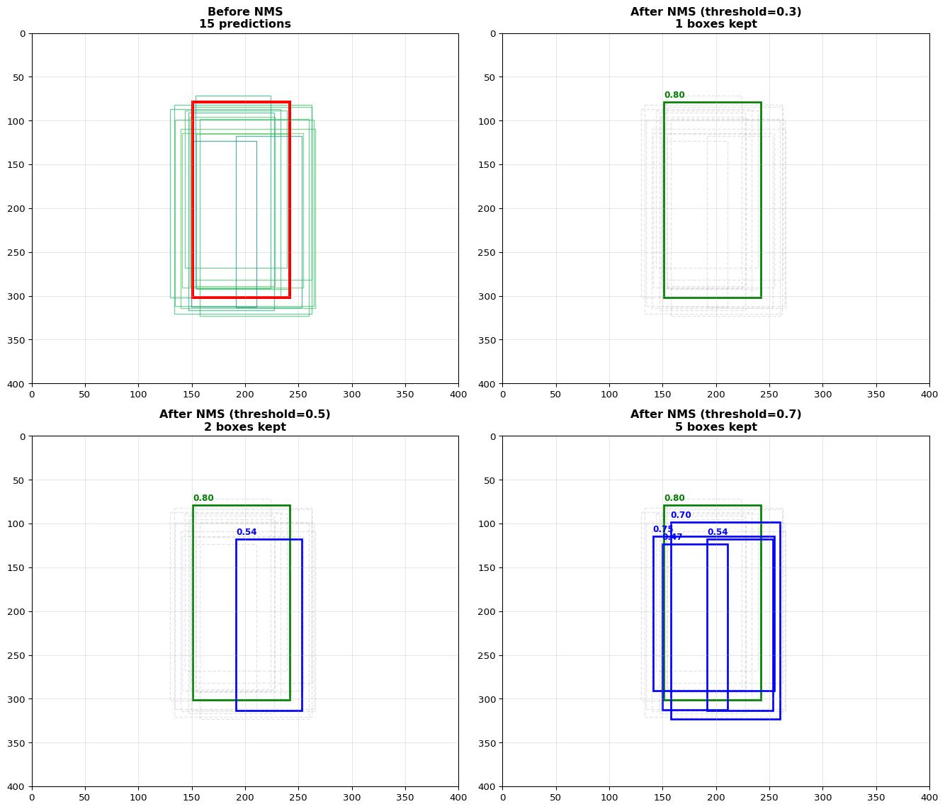
YOLO predicts 1000+ bounding boxes per image. Most overlap or have low confidence. NMS filters redundant boxes:

Sort all boxes by confidence score
Take the highest-confidence box
Remove all boxes with IoU > threshold (0.5 typically) with the selected box
Repeat on remaining boxes

NMS Threshold Trade-off: Low threshold (0.3) keeps only very distinct boxes—good for separate objects, bad for crowds. High threshold (0.7) keeps overlapping boxes—good for dense scenes, but produces duplicates.

Edge Optimization Pipeline

Image Preprocessing: Resize to 416×416 or 224×224 (smaller = faster but less detail)
Quantization: INT8 TFLite model (4× smaller, 3-5× faster)
NMS Tuning: Increase confidence threshold (0.25 → 0.5) to filter weak predictions
Frame Skipping: Process every 2nd or 3rd frame for smoother video
ROI Cropping: If detecting objects in a fixed area (e.g., door entrance), crop image first

Key Concepts at a Glance

Core Concepts

Single-Shot Detection: YOLO predicts boxes and classes in one pass (vs two-stage R-CNN)
Grid-Based Prediction: Divide image into SxS grid; each cell predicts B boxes
Anchor Boxes: Pre-defined box shapes; model predicts offsets from anchors
Confidence Score: P(object) × IoU—suppresses background predictions
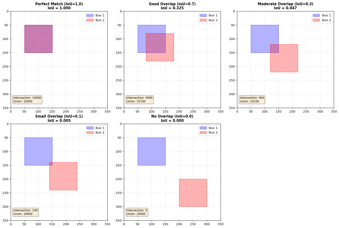
IoU (Intersection over Union): Overlap metric; IoU = Area(A ∩ B) / Area(A ∪ B)
NMS (Non-Maximum Suppression): Filters duplicate boxes by removing overlapping predictions
mAP (mean Average Precision): Standard metric for object detection accuracy (higher = better)

Common Pitfalls

Mistakes to Avoid

Forgetting Input Normalization: YOLO expects pixel values in [0, 1] range. If you forget to divide by 255.0, predictions will be garbage. Always check: input_data = input_data.astype(np.float32) / 255.0
Mismatched Anchor Boxes: If you train a custom YOLO model with K-means-derived anchors but deploy with default COCO anchors, accuracy drops dramatically. Always use the same anchors for training and inference.
Setting NMS Threshold Too Low: NMS threshold = 0.1 removes almost all boxes, even correct ones. Start with 0.5 and tune based on your use case (dense scenes need higher thresholds).
Ignoring Aspect Ratio in Resize: If your input image is 1920×1080 and you resize to 416×416 without padding, objects appear squashed. Use letterbox resizing: pad to square first, then resize.
Using Full YOLO on ESP32: Full YOLOv3 requires 250MB+ RAM. ESP32 has 520KB. Even Tiny-YOLO needs careful optimization. Use YOLO-Nano or simpler models (MobileNet-SSD) for MCU deployment.
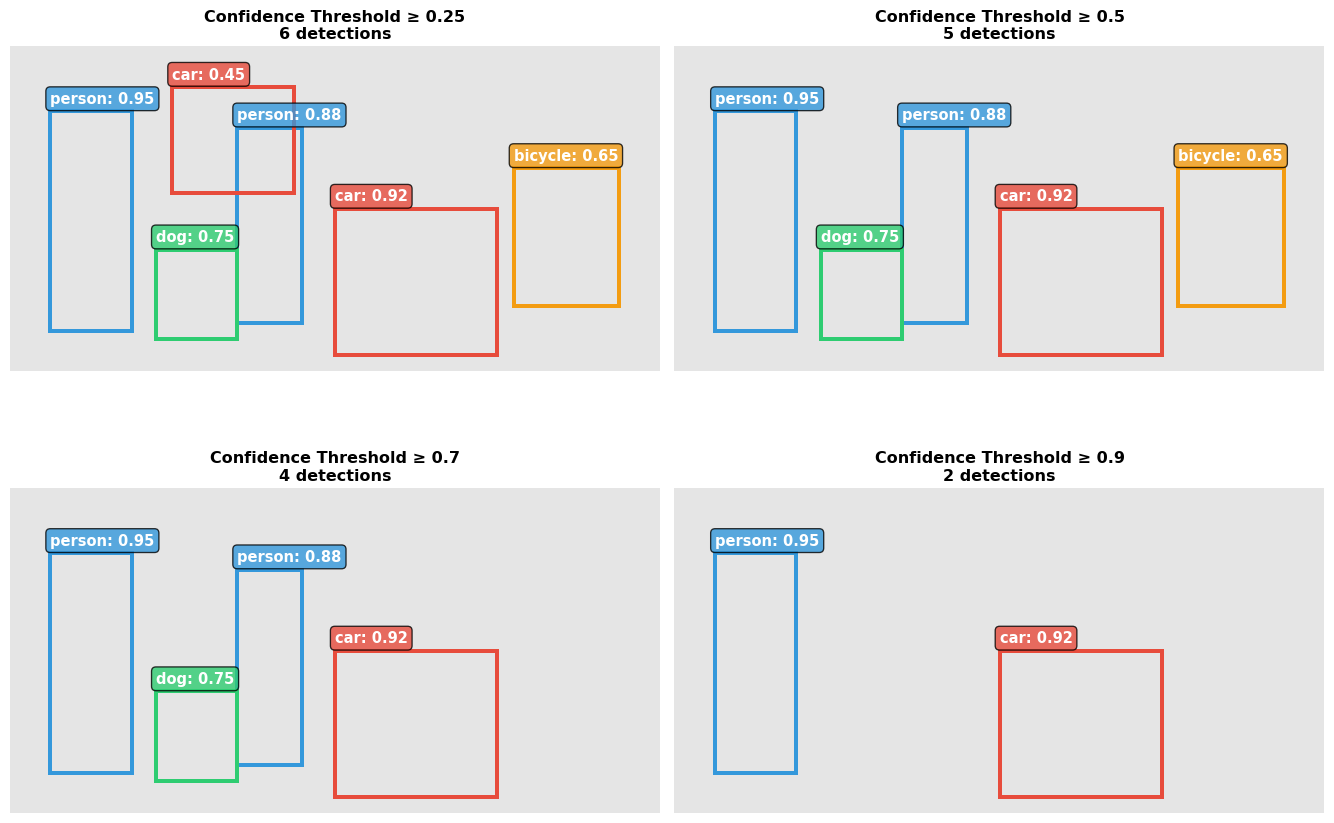
Not Tuning Confidence Threshold for Edge: Cloud deployments often use confidence = 0.25. For edge, raise to 0.5-0.7 to filter weak predictions and reduce post-processing load (faster inference).

Quick Reference

TFLite YOLO Inference Pipeline

import numpy as np
import cv2
import tensorflow as tf

# Load TFLite model
interpreter = tf.lite.Interpreter(model_path="tiny_yolo_v3.tflite")
interpreter.allocate_tensors()

input_details = interpreter.get_input_details()
output_details = interpreter.get_output_details()

# Preprocess image
img = cv2.imread("image.jpg")
img_resized = cv2.resize(img, (416, 416))
input_data = np.expand_dims(img_resized, axis=0).astype(np.float32) / 255.0

# Run inference
interpreter.set_tensor(input_details[0]['index'], input_data)
interpreter.invoke()
predictions = interpreter.get_tensor(output_details[0]['index'])

# Post-process: NMS, confidence filtering
boxes, scores, classes = post_process_yolo(predictions, conf_thresh=0.5, nms_thresh=0.5)

Non-Maximum Suppression (NumPy)

def nms(boxes, scores, iou_threshold=0.5):
    """
    boxes: Nx4 array of [x1, y1, x2, y2]
    scores: N array of confidence scores
    """
    indices = np.argsort(scores)[::-1]  # Sort descending
    keep = []

    while len(indices) > 0:
        current = indices[0]
        keep.append(current)

        # Compute IoU of current box with all others
        ious = compute_iou(boxes[current], boxes[indices[1:]])

        # Keep only boxes with IoU < threshold
        indices = indices[1:][ious < iou_threshold]

    return keep

IoU Calculation

def compute_iou(box1, box2):
    """Intersection over Union"""
    x1 = max(box1[0], box2[0])
    y1 = max(box1[1], box2[1])
    x2 = min(box1[2], box2[2])
    y2 = min(box1[3], box2[3])

    intersection = max(0, x2 - x1) * max(0, y2 - y1)
    area1 = (box1[2] - box1[0]) * (box1[3] - box1[1])
    area2 = (box2[2] - box2[0]) * (box2[3] - box2[1])
    union = area1 + area2 - intersection

    return intersection / union if union > 0 else 0

Edge Device Performance Benchmarks

Device	Model	Input Size	FPS	Power	Use Case
Raspberry Pi 4	Tiny-YOLO INT8	416×416	5	3W	Security camera
Raspberry Pi Zero	YOLO-Nano INT8	224×224	1	0.5W	Doorbell cam
ESP32-CAM	MobileNet-SSD	160×160	2	0.2W	IoT sensor
Coral USB	Tiny-YOLO EdgeTPU	416×416	30	2W	Drone vision

Accuracy Metrics

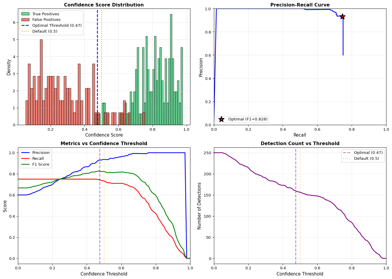
Precision: Of all boxes predicted as “person”, what % are actually people?

Recall: Of all actual people in the image, what % did we detect?

mAP (mean Average Precision): Average precision across all classes and IoU thresholds. Industry standard for object detection.

\[\text{mAP} = \frac{1}{N} \sum_{i=1}^{N} AP_i\]

where $AP_i$ is the average precision for class $i$ computed from the precision-recall curve.

Related Concepts in PDF Chapter 16

Section 16.2: YOLO architecture and single-shot detection explanation
Section 16.3: Anchor boxes and grid-based prediction mechanism
Section 16.4: TFLite conversion and INT8 quantization for Tiny-YOLO
Section 16.5: NMS algorithm implementation and threshold tuning
Section 16.6: Raspberry Pi deployment with picamera integration
Section 16.7: ESP32-CAM deployment and optimization techniques

Self-Assessment Checkpoints

Test your understanding before proceeding to the exercises.

Question 1: Calculate the total output size for YOLO with a 13×13 grid, 5 anchor boxes per cell, and 80 classes.

Answer: Output size = Grid_Height × Grid_Width × Anchors × (Box_coords + Confidence + Classes) = 13 × 13 × 5 × (4 + 1 + 80) = 13 × 13 × 5 × 85 = 71,825 values. Each grid cell predicts 5 bounding boxes, and for each box: 4 coordinates (x, y, width, height), 1 confidence score (objectness), and 80 class probabilities. This tensor must fit in memory during inference, which is why Tiny-YOLO uses smaller grids (e.g., 7×7) to reduce memory requirements for edge devices.

Question 2: Why does YOLO use anchor boxes instead of directly predicting bounding box dimensions?

Answer: Anchor boxes stabilize training by providing reasonable initial box shapes. Without anchors, the network must learn box sizes from scratch—extremely difficult because bounding boxes vary by orders of magnitude (tiny person 30×100px vs large car 300×200px). Anchors are pre-computed from training data using K-means clustering to find common object shapes (tall/narrow for people, wide/short for cars, square for faces). The network then predicts small offsets from these anchors, making learning easier. This is why training a custom YOLO model requires generating anchors from your specific dataset—using COCO anchors for different object types reduces accuracy.

Question 3: Explain the NMS threshold trade-off. What happens with threshold=0.1 vs threshold=0.9?

Answer: NMS threshold = 0.1: Very aggressive filtering. Only keeps boxes with IoU < 0.1 (barely overlapping). Removes almost all duplicate predictions, but also removes valid overlapping objects (e.g., people in a crowd, stacked boxes). Result: misses detections in dense scenes. NMS threshold = 0.9: Very lenient filtering. Keeps boxes even with 90% overlap. Preserves detections in crowded scenes but produces many duplicate boxes around the same object. Result: multiple boxes per object. Sweet spot: 0.4-0.6 for general use. Tune based on application: use 0.7-0.8 for crowd detection, 0.3-0.5 for sparse scenes with distinct objects.

Question 4: Your Raspberry Pi 4 runs Tiny-YOLO at 5 FPS. What optimizations can improve this to 10+ FPS?

Answer: (1) Reduce input resolution: 416×416 → 224×224 gives 4× pixel reduction = ~2× speedup (less accurate for small objects), (2) INT8 quantization: Convert to TFLite INT8 model for 3-5× speedup with 2-3% accuracy loss, (3) Frame skipping: Process every 2nd frame, interpolate predictions = 2× effective FPS, (4) ROI cropping: If objects appear in fixed regions (doorway, road), crop to region of interest before inference = smaller input = faster, (5) Use TPU/Coral accelerator: Adds ~$25 USB accelerator for 10-30× speedup to 50-150 FPS. Combined: 224×224 + INT8 + frame skip = potential 20+ FPS on Pi 4.

Question 5: Can you run full YOLOv3 (62M parameters, 140 GFLOPS) on an ESP32? Why or why not?

Answer: No, absolutely not. The math is prohibitive: Memory: YOLOv3 requires ~250 MB just for model weights (62M params × 4 bytes). ESP32 has 520 KB SRAM (500× too small). Even INT8 quantized (62 MB) won’t fit. Computation: 140 GFLOPS at 240 MHz dual-core ≈ 300 seconds per frame (0.003 FPS). ESP32 is for ultra-lightweight models. Options for ESP32: (1) YOLO-Nano (4M params, 2.2 GFLOPS) might work with aggressive quantization, (2) MobileNet-SSD (5M params) is better suited, (3) Pre-processing only: Run YOLO on Pi/cloud, ESP32 handles camera and sends images. For object detection on MCUs, expect 10-20% accuracy of full models—acceptable for simple tasks (person detection, yes/no classification).

Interactive Notebook

The notebook below contains runnable code for all Level 1 activities.

LAB16: Computer Vision with YOLO for Edge Devices

Learning Objectives: - Understand object detection architectures (one-stage vs two-stage) - Implement YOLO object detection using OpenCV DNN - Apply Non-Maximum Suppression (NMS) for filtering detections - Optimize for edge deployment (Tiny-YOLO, MobileNet-SSD) - Measure and improve inference performance

Three-Tier Approach: - Level 1 (This Notebook): Run YOLO on static images - Level 2 (Simulator): Process video streams on laptop/desktop - Level 3 (Device): Deploy on Raspberry Pi with camera

1. Setup

📚 Theory: Object Detection Fundamentals

Object detection is fundamentally different from image classification.

Classification vs Detection vs Segmentation

Classification:               Detection:                    Segmentation:
┌─────────────────┐          ┌─────────────────┐          ┌─────────────────┐
│  🐕 🐈           │          │  ┌───┐          │          │  █████          │
│                 │          │  │🐕│  ┌──┐     │          │  ████████       │
│                 │          │  └───┘  │🐈│     │          │  ▓▓▓▓▓▓▓▓▓▓     │
│                 │          │         └──┘     │          │       ░░░░░░░░  │
└─────────────────┘          └─────────────────┘          └─────────────────┘
Output: "dog"                Output: boxes +              Output: pixel-wise
(single label)               labels                       masks

Detection Output Format

Each detection consists of: - Bounding box: $(x, y, w, h)$ or $(x_{min}, y_{min}, x_{max}, y_{max})$ - Class label: e.g., “person”, “car”, “dog” - Confidence score: probability $p \in [0, 1]$

Two-Stage vs One-Stage Detectors

Two-Stage (R-CNN family):        One-Stage (YOLO, SSD):

Image → Region      → Classify   Image → Single        → Boxes +
        Proposals      Regions          Forward Pass      Classes
        (RPN)                           
┌────┐   ┌────┐   ┌────┐        ┌────┐   ┌────────┐
│    │ → │RP │ → │CNN │        │    │ → │ CNN    │
│    │   │   │   │    │        │    │   │        │
└────┘   └────┘   └────┘        └────┘   └────────┘
                                          ↓ Direct
  Slow but accurate              Fast but less accurate
  ~5 FPS                         ~30+ FPS

Comparison

Approach	Speed	Accuracy	Edge Suitable
Faster R-CNN	Slow	High	No
YOLO	Fast	Medium-High	Yes
SSD	Fast	Medium	Yes
MobileNet-SSD	Very Fast	Medium	Excellent

2. Object Detection Fundamentals

Classification vs Detection

Classification: “Is there a dog in this image?” (one label per image)
Detection: “Where are all the dogs?” (multiple bounding boxes + labels)

YOLO: You Only Look Once

YOLO processes the entire image in a single forward pass: 1. Divide image into grid cells 2. Each cell predicts bounding boxes + class probabilities 3. Apply Non-Maximum Suppression to filter duplicates

📚 Theory: YOLO Architecture

YOLO (You Only Look Once) revolutionized object detection by treating it as a regression problem.

Grid-Based Detection

Input Image (416×416)         Grid (13×13)              Predictions
┌───────────────────┐        ┌─┬─┬─┬─┬─┬─┬─┐          Each cell predicts:
│                   │        ├─┼─┼─┼─┼─┼─┼─┤          • B bounding boxes
│     ┌────┐        │   →    ├─┼─┼─┼─●─┼─┼─┤   →      • C class probabilities
│     │ 🚗 │        │        ├─┼─┼─┼─┼─┼─┼─┤          
│     └────┘        │        ├─┼─┼─┼─┼─┼─┼─┤          Output: S×S×(B×5 + C)
│                   │        └─┴─┴─┴─┴─┴─┴─┘          
└───────────────────┘                                 For YOLOv3-Tiny:
                                                      13×13×(3×(4+1+80))
Cell responsible for                                  = 13×13×255
object if center falls within it

Bounding Box Prediction

Each bounding box predicts 5 values:

$\begin{aligned} b_x &= \sigma(t_x) + c_x & \text{(center x relative to grid cell)}\\ b_y &= \sigma(t_y) + c_y & \text{(center y relative to grid cell)}\\ b_w &= p_w \cdot e^{t_w} & \text{(width relative to anchor)}\\ b_h &= p_h \cdot e^{t_h} & \text{(height relative to anchor)}\\ \text{conf} &= \sigma(t_o) & \text{(objectness score)} \end{aligned}$

Where $\sigma$ is the sigmoid function, $c_x, c_y$ are cell coordinates, and $p_w, p_h$ are anchor dimensions.

Bounding Box Parameterization:

     ┌─────────────────────┐
     │      Grid Cell      │
     │   ┌───────────┐     │
     │   │           │     │
     │   │    ●(bx,by)     │ ← Center predicted
     │   │           │     │   relative to cell
     │   └───────────┘     │
     │        bw           │
     └─────────────────────┘
           bh

Anchor Boxes

Predefined aspect ratios for common object shapes:

Anchor Box Examples:
┌─────┐   ┌───────────┐   ┌───┐
│     │   │           │   │   │
│     │   │           │   │   │
│     │   │           │   │   │
│     │   └───────────┘   │   │
│     │      1:3 wide     │   │
└─────┘                   │   │
 1:1                      │   │
square                    └───┘
                          3:1 tall

YOLOv3-Tiny anchors (from k-means on COCO):
10×14, 23×27, 37×58, 81×82, 135×169, 344×319

YOLOv3-Tiny Architecture

Input: 416×416×3
       │
       ▼
┌─────────────────┐
│ 7 Conv Layers   │  Backbone (feature extraction)
│ + MaxPool       │  Darknet-53 simplified
└────────┬────────┘
         │
    ┌────┴────┐
    ▼         ▼
┌───────┐ ┌───────┐
│13×13  │ │26×26  │  Multi-scale predictions
│×255   │ │×255   │  
└───────┘ └───────┘
 Large      Small
 objects    objects

3. Download Model Files

4. Load YOLO Network

5. Download Test Images

6. YOLO Detection Pipeline

📚 Theory: Detection Pipeline

Image Preprocessing

YOLO expects specific input format:

Original Image         Preprocessing Steps         Network Input
┌─────────────┐                                   ┌─────────────┐
│ Variable    │  1. Resize to 416×416             │ 416×416×3   │
│ size        │  2. Normalize [0,1]               │ Float32     │
│ uint8 BGR   │  3. BGR → RGB                     │ RGB         │
│             │  4. Add batch dimension           │ (1,3,416,416)│
└─────────────┘                                   └─────────────┘

Blob Creation

OpenCV creates a “blob” for DNN input:

blob = cv2.dnn.blobFromImage(
    image,           # Input image (BGR)
    1/255.0,         # Scale factor (normalize to [0,1])
    (416, 416),      # Output size
    swapRB=True,     # BGR → RGB
    crop=False       # Resize without cropping
)
# Output shape: (1, 3, 416, 416)

Output Interpretation

YOLO output is a tensor where each row is a detection:

Detection Row Format:
┌────┬────┬────┬────┬──────┬─────────────────────┐
│ cx │ cy │ w  │ h  │ conf │ class_0 ... class_N │
└────┴────┴────┴────┴──────┴─────────────────────┘
  │     │    │    │     │            │
  └─────┴────┴────┘     │            └── Class probabilities
    Normalized          │
    [0,1] coords        └── Objectness score

Coordinate Conversion

Convert from YOLO format to pixel coordinates:

$\begin{aligned} \text{center\_x} &= \text{cx} \times W_{image} \\ \text{center\_y} &= \text{cy} \times H_{image} \\ \text{width} &= w \times W_{image} \\ \text{height} &= h \times H_{image} \\ x_{min} &= \text{center\_x} - \frac{\text{width}}{2} \end{aligned}$

7. Visualize Detections

8. Understanding Non-Maximum Suppression (NMS)

YOLO produces multiple overlapping detections for the same object. NMS filters them:

Sort detections by confidence
Keep highest confidence detection
Remove all detections with IoU > threshold
Repeat for remaining detections

📚 Theory: Non-Maximum Suppression (NMS)

The Problem: Multiple Detections

Multiple grid cells and anchor boxes may detect the same object:

Before NMS:                    After NMS:
┌──────────────────────┐      ┌──────────────────────┐
│  ┌───────────┐       │      │                      │
│  │┌─────────┐│       │      │  ┌─────────┐         │
│  ││┌───────┐││ 🚗    │  →   │  │ 🚗 95%  │         │
│  │││ 🚗    │││       │      │  └─────────┘         │
│  ││└───────┘││       │      │                      │
│  │└─────────┘│       │      │                      │
│  └───────────┘       │      │                      │
└──────────────────────┘      └──────────────────────┘
   3 overlapping boxes            1 final detection

Intersection over Union (IoU)

IoU measures overlap between two boxes:

$IoU = \frac{\text{Area of Intersection}}{\text{Area of Union}} = \frac{A \cap B}{A \cup B}$

IoU Calculation:
                                          
  ┌─────────┐            ┌───┬─────┬───┐
  │    A    │            │   │█████│   │
  │    ┌────┼───┐        │ A │█Int█│ B │
  └────┼────┘   │   →    │   │█████│   │
       │    B   │        └───┴─────┴───┘
       └────────┘        
                         IoU = Int / (A + B - Int)

IoU Interpretation

IoU Value	Meaning
0	No overlap
0.3	Slight overlap
0.5	Moderate overlap
0.7	Significant overlap
1.0	Perfect overlap

NMS Algorithm

Input: B = boxes, S = scores, threshold
Output: D = kept detections

D = []
while B not empty:
    m = argmax(S)           # Find highest confidence
    D.append(B[m])          # Keep it
    B.remove(m)             # Remove from list
    
    for each remaining box b in B:
        if IoU(B[m], b) > threshold:
            B.remove(b)     # Remove overlapping boxes

return D

Typical NMS Thresholds

Application	IoU Threshold	Notes
General detection	0.4-0.5	Standard
Crowded scenes	0.6-0.7	More boxes kept
High precision	0.3-0.4	Fewer duplicates

9. Performance Benchmarking

10. Edge Deployment Considerations

Model Size Comparison

Model	Size	Params	Pi4 FPS	Accuracy (mAP)
YOLOv3	237 MB	65M	<1	57%
YOLOv3-Tiny	34 MB	8.8M	2-4	33%
MobileNet-SSD	23 MB	6.8M	4-6	21%

Optimization Tips

Use Tiny-YOLO instead of full YOLO
Reduce input resolution (320x320 vs 416x416)
Use hardware acceleration (Coral TPU, OpenCV NEON)

📚 Theory: Edge Optimization for Object Detection

Computation Cost Analysis

Inference cost is dominated by convolutions:

$\text{FLOPs} = 2 \times C_{in} \times C_{out} \times K^2 \times H_{out} \times W_{out}$

For YOLOv3-Tiny at 416×416: - Total: ~5.6 billion FLOPs - Raspberry Pi 4: ~10 GFLOPS (theoretical) - Expected: ~1-2 FPS (real-world)

Resolution Trade-off

Input Resolution vs Performance:

Resolution │ FLOPs      │ Small Objects │ FPS (Pi4)
───────────┼────────────┼───────────────┼──────────
608×608    │ 11.5B      │ Best          │ <1
416×416    │ 5.6B       │ Good          │ 2-3
320×320    │ 3.3B       │ Medium        │ 4-5
224×224    │ 1.6B       │ Poor          │ 8-10

Hardware Acceleration Options

┌─────────────────────────────────────────────────────────────────┐
│                    ACCELERATION OPTIONS                         │
├────────────────┬──────────────┬──────────────┬─────────────────┤
│   Device       │   Speedup    │    Cost      │   Power         │
├────────────────┼──────────────┼──────────────┼─────────────────┤
│ CPU (ARM)      │ 1x (baseline)│ $0           │ ~3W             │
│ NEON SIMD      │ 1.5-2x       │ $0           │ ~3W             │
│ GPU (Pi)       │ 1.2-1.5x     │ $0           │ ~4W             │
│ Coral TPU      │ 10-20x       │ $60          │ ~2W             │
│ NVIDIA Jetson  │ 20-50x       │ $100-500     │ 10-30W          │
└────────────────┴──────────────┴──────────────┴─────────────────┘

Quantization Impact

Precision	Model Size	Speed	mAP Change
FP32	100%	1x	0%
FP16	50%	1.5-2x	-0.5%
INT8	25%	2-4x	-1-2%

Memory Budget (Raspberry Pi)

Pi 4 (4GB RAM) Memory Allocation:
┌────────────────────────────────────────────────────────────┐
│ OS + Services:     ~500 MB                                 │
├────────────────────────────────────────────────────────────┤
│ Model weights:     ~35 MB (YOLOv3-Tiny)                   │
├────────────────────────────────────────────────────────────┤
│ Input image:       ~2 MB (1920×1080×3)                    │
├────────────────────────────────────────────────────────────┤
│ Inference buffers: ~50-100 MB (activations)               │
├────────────────────────────────────────────────────────────┤
│ Available:         ~3.3 GB                                │
└────────────────────────────────────────────────────────────┘

📚 Summary: Key Formulas and Concepts

YOLO Detection

Box prediction: $b_x = \sigma(t_x) + c_x, \quad b_w = p_w \cdot e^{t_w}$

Objectness score: $\text{conf} = P(\text{object}) \times IoU_{pred}^{truth}$

Intersection over Union

$IoU = \frac{\text{Area}(A \cap B)}{\text{Area}(A \cup B)}$

Computational Cost

$\text{FLOPs}_{conv} \propto C_{in} \times C_{out} \times K^2 \times H \times W$

Edge Deployment Guidelines

Requirement	Recommendation
>10 FPS	Use MobileNet-SSD, 320px input
3-10 FPS	Use YOLOv3-Tiny, consider TPU
High accuracy	Use full YOLOv3 with Jetson
Low power	INT8 quantization + TPU

Detection Pipeline

Image → Preprocess → CNN → Parse Output → NMS → Final Detections
        (resize,      ↓     (threshold,   ↓
         normalize)         convert)      (filter duplicates)

11. Checkpoint Questions

Why does YOLO produce multiple detections for the same object?
- Hint: Think about grid cells and anchor boxes
What is the purpose of Non-Maximum Suppression?
- Hint: Removes duplicates based on IoU
How does reducing input size affect detection?
- Speed: Increases (fewer computations)
- Small object detection: Decreases (less resolution)
For a warehouse robot detecting packages on a conveyor, would you choose YOLOv3 (0.5 FPS, 57% mAP) or Tiny-YOLO (4 FPS, 33% mAP)? Why?
- Hint: Consider real-time requirements vs accuracy needs

12. Next Steps

Level 2: Video Stream Processing

cap = cv2.VideoCapture(0)  # Webcam
while True:
    ret, frame = cap.read()
    boxes, confs, ids = detect_objects(frame, net, output_layers)
    result = draw_detections(frame, boxes, confs, ids, CLASSES)
    cv2.imshow('YOLO', result)
    if cv2.waitKey(1) == ord('q'):
        break

Level 3: Raspberry Pi Deployment

See textbook Chapter 16 for: - Pi Camera integration - Threading for better FPS - Coral TPU acceleration

Three-Tier Activities

Environment: local Jupyter or Colab, no hardware required.

Suggested workflow:

Use the notebook to run YOLO/Tiny-YOLO on static images:
- visualise bounding boxes, labels, and confidence scores
- experiment with confidence and NMS thresholds.
Inspect model size and approximate FLOPs or parameter counts.
Compare at least two configurations (e.g., full vs Tiny, 416×416 vs 320×320) and note the expected FPS difference on edge hardware.

Here you build and profile a full video pipeline on a laptop or Raspberry Pi before deploying to a dedicated edge device.

Use the lab notebook or a standalone script to:
- open a webcam or video file
- apply YOLO/Tiny-YOLO frame-by-frame
- measure FPS and latency.
Use these interactive tools to deepen understanding:
- Our NMS Visualization to see how NMS removes duplicate boxes.
- Netron to inspect model architecture and layer shapes.
- Ultralytics HUB (optional) to train/test custom models in the cloud and export edge-suitable variants.

Capture simple metrics (FPS, CPU utilisation where possible) and decide which model/resolution combination is acceptable for your target scenario.

Deploy Tiny-YOLO (or a similar lightweight detector) on Raspberry Pi with a camera module.

Install OpenCV and the required YOLO/Tiny-YOLO weights/config on the Pi.
Implement a minimal detection loop:
- capture frames from Pi Camera,
- run Tiny-YOLO with a reduced input size (e.g., 320×320),
- draw detections and print FPS.
Record:
- typical and worst-case FPS,
- CPU utilisation,
- any thermal or stability issues over a multi-minute run.
Relate these findings back to course themes:
- would this detector meet the latency requirements of your application?
- what happens if you reduce classes, resolution, or move to an accelerator?

Try It Yourself: Executable Python Examples

Below are interactive Python examples you can run directly in this Quarto document to explore YOLO object detection concepts.

Example 1: IoU (Intersection over Union) Calculation

Code

import numpy as np
import matplotlib.pyplot as plt
import matplotlib.patches as patches

def calculate_iou(box1, box2):
    """
    Calculate Intersection over Union (IoU) between two bounding boxes

    Args:
        box1, box2: [x1, y1, x2, y2] format where (x1,y1) is top-left, (x2,y2) is bottom-right

    Returns:
        IoU value between 0 and 1
    """
    # Calculate intersection coordinates
    x1_inter = max(box1[0], box2[0])
    y1_inter = max(box1[1], box2[1])
    x2_inter = min(box1[2], box2[2])
    y2_inter = min(box1[3], box2[3])

    # Calculate intersection area
    if x2_inter < x1_inter or y2_inter < y1_inter:
        intersection = 0
    else:
        intersection = (x2_inter - x1_inter) * (y2_inter - y1_inter)

    # Calculate union area
    area1 = (box1[2] - box1[0]) * (box1[3] - box1[1])
    area2 = (box2[2] - box2[0]) * (box2[3] - box2[1])
    union = area1 + area2 - intersection

    # Calculate IoU
    iou = intersection / union if union > 0 else 0

    return iou, intersection, union

# Example bounding boxes
boxes_examples = [
    {
        'name': 'Perfect Match (IoU=1.0)',
        'box1': [50, 50, 150, 150],
        'box2': [50, 50, 150, 150],
    },
    {
        'name': 'Good Overlap (IoU≈0.7)',
        'box1': [50, 50, 150, 150],
        'box2': [80, 80, 180, 180],
    },
    {
        'name': 'Moderate Overlap (IoU≈0.3)',
        'box1': [50, 50, 150, 150],
        'box2': [120, 120, 220, 220],
    },
    {
        'name': 'Small Overlap (IoU≈0.1)',
        'box1': [50, 50, 150, 150],
        'box2': [140, 140, 240, 240],
    },
    {
        'name': 'No Overlap (IoU=0.0)',
        'box1': [50, 50, 150, 150],
        'box2': [200, 200, 300, 300],
    },
]

# Visualization
fig, axes = plt.subplots(2, 3, figsize=(15, 10))
axes = axes.flatten()

for idx, example in enumerate(boxes_examples):
    ax = axes[idx]

    box1 = example['box1']
    box2 = example['box2']
    iou, intersection, union = calculate_iou(box1, box2)

    # Create rectangles
    rect1 = patches.Rectangle((box1[0], box1[1]), box1[2]-box1[0], box1[3]-box1[1],
                               linewidth=2, edgecolor='blue', facecolor='blue',
                               alpha=0.3, label='Box 1')
    rect2 = patches.Rectangle((box2[0], box2[1]), box2[2]-box2[0], box2[3]-box2[1],
                               linewidth=2, edgecolor='red', facecolor='red',
                               alpha=0.3, label='Box 2')

    ax.add_patch(rect1)
    ax.add_patch(rect2)

    # Set plot properties
    ax.set_xlim(0, 350)
    ax.set_ylim(0, 350)
    ax.set_aspect('equal')
    ax.invert_yaxis()
    ax.grid(True, alpha=0.3)
    ax.set_title(f"{example['name']}\nIoU = {iou:.3f}", fontsize=11, fontweight='bold')
    ax.legend(loc='upper right')

    # Add IoU calculation text
    text = f"Intersection: {intersection:.0f}\nUnion: {union:.0f}"
    ax.text(10, 330, text, fontsize=9,
            bbox=dict(boxstyle='round', facecolor='wheat', alpha=0.5))

# Hide unused subplot
axes[-1].axis('off')

plt.tight_layout()
plt.show()

# Print detailed calculations
print("IoU Calculation Examples")
print("="*80)

for example in boxes_examples:
    box1 = example['box1']
    box2 = example['box2']
    iou, intersection, union = calculate_iou(box1, box2)

    print(f"\n{example['name']}:")
    print(f"  Box 1: {box1}")
    print(f"  Box 2: {box2}")
    print(f"  Intersection area: {intersection:.0f}")
    print(f"  Union area: {union:.0f}")
    print(f"  IoU: {iou:.3f}")

print("\n" + "="*80)
print("IoU Interpretation:")
print("  • IoU > 0.5: Good match (typically used for 'correct' detection)")
print("  • IoU > 0.7: Strong match")
print("  • IoU > 0.9: Almost perfect match")
print("  • IoU = 1.0: Perfect match (identical boxes)")

IoU Calculation Examples
================================================================================

Perfect Match (IoU=1.0):
  Box 1: [50, 50, 150, 150]
  Box 2: [50, 50, 150, 150]
  Intersection area: 10000
  Union area: 10000
  IoU: 1.000

Good Overlap (IoU≈0.7):
  Box 1: [50, 50, 150, 150]
  Box 2: [80, 80, 180, 180]
  Intersection area: 4900
  Union area: 15100
  IoU: 0.325

Moderate Overlap (IoU≈0.3):
  Box 1: [50, 50, 150, 150]
  Box 2: [120, 120, 220, 220]
  Intersection area: 900
  Union area: 19100
  IoU: 0.047

Small Overlap (IoU≈0.1):
  Box 1: [50, 50, 150, 150]
  Box 2: [140, 140, 240, 240]
  Intersection area: 100
  Union area: 19900
  IoU: 0.005

No Overlap (IoU=0.0):
  Box 1: [50, 50, 150, 150]
  Box 2: [200, 200, 300, 300]
  Intersection area: 0
  Union area: 20000
  IoU: 0.000

================================================================================
IoU Interpretation:
  • IoU > 0.5: Good match (typically used for 'correct' detection)
  • IoU > 0.7: Strong match
  • IoU > 0.9: Almost perfect match
  • IoU = 1.0: Perfect match (identical boxes)

Example 2: Non-Maximum Suppression (NMS) Demo

Code

import numpy as np
import matplotlib.pyplot as plt
import matplotlib.patches as patches

def nms(boxes, scores, iou_threshold=0.5):
    """
    Perform Non-Maximum Suppression on bounding boxes

    Args:
        boxes: numpy array of shape (N, 4), each row is [x1, y1, x2, y2]
        scores: numpy array of shape (N,), confidence scores
        iou_threshold: IoU threshold for suppression

    Returns:
        List of indices of boxes to keep
    """
    if len(boxes) == 0:
        return []

    # Sort boxes by score (descending)
    indices = np.argsort(scores)[::-1]
    keep = []

    while len(indices) > 0:
        # Take box with highest score
        current_idx = indices[0]
        keep.append(current_idx)

        if len(indices) == 1:
            break

        # Calculate IoU with all other boxes
        current_box = boxes[current_idx]
        other_boxes = boxes[indices[1:]]

        ious = np.array([calculate_iou(current_box, box)[0] for box in other_boxes])

        # Keep only boxes with IoU below threshold
        mask = ious < iou_threshold
        indices = indices[1:][mask]

    return keep

# Generate simulated detections for a person
np.random.seed(42)

# True object location
true_box = [150, 100, 250, 300]

# Generate multiple overlapping predictions (as YOLO would produce)
num_predictions = 15
boxes = []
scores = []

for i in range(num_predictions):
    # Add noise to true box
    noise = np.random.randn(4) * 15
    noisy_box = [
        max(0, true_box[0] + noise[0]),
        max(0, true_box[1] + noise[1]),
        min(400, true_box[2] + noise[2]),
        min(400, true_box[3] + noise[3])
    ]
    boxes.append(noisy_box)

    # Generate confidence score (higher for boxes closer to true box)
    iou_with_true = calculate_iou(noisy_box, true_box)[0]
    score = iou_with_true * 0.9 + np.random.rand() * 0.1
    scores.append(score)

boxes = np.array(boxes)
scores = np.array(scores)

# Apply NMS with different thresholds
thresholds = [0.3, 0.5, 0.7]
nms_results = {}

for threshold in thresholds:
    kept_indices = nms(boxes, scores, iou_threshold=threshold)
    nms_results[threshold] = kept_indices

# Visualization
fig, axes = plt.subplots(2, 2, figsize=(14, 12))
axes = axes.flatten()

# Plot 1: All predictions before NMS
ax = axes[0]
for i, (box, score) in enumerate(zip(boxes, scores)):
    color = plt.cm.viridis(score)
    rect = patches.Rectangle((box[0], box[1]), box[2]-box[0], box[3]-box[1],
                             linewidth=1, edgecolor=color, facecolor='none',
                             alpha=0.7)
    ax.add_patch(rect)

# Highlight highest confidence box
max_idx = np.argmax(scores)
max_box = boxes[max_idx]
rect = patches.Rectangle((max_box[0], max_box[1]),
                         max_box[2]-max_box[0], max_box[3]-max_box[1],
                         linewidth=3, edgecolor='red', facecolor='none')
ax.add_patch(rect)

ax.set_xlim(0, 400)
ax.set_ylim(0, 400)
ax.invert_yaxis()
ax.set_title(f'Before NMS\n{num_predictions} predictions', fontsize=12, fontweight='bold')
ax.grid(True, alpha=0.3)

# Plot 2-4: After NMS with different thresholds
for idx, threshold in enumerate(thresholds, start=1):
    ax = axes[idx]
    kept_indices = nms_results[threshold]

    # Draw all boxes (faded)
    for box in boxes:
        rect = patches.Rectangle((box[0], box[1]), box[2]-box[0], box[3]-box[1],
                                 linewidth=1, edgecolor='gray', facecolor='none',
                                 alpha=0.2, linestyle='--')
        ax.add_patch(rect)

    # Draw kept boxes
    for i in kept_indices:
        box = boxes[i]
        score = scores[i]
        color = 'green' if i == np.argmax(scores) else 'blue'
        rect = patches.Rectangle((box[0], box[1]), box[2]-box[0], box[3]-box[1],
                                 linewidth=2, edgecolor=color, facecolor='none')
        ax.add_patch(rect)
        ax.text(box[0], box[1]-5, f'{score:.2f}', fontsize=9,
                color=color, fontweight='bold')

    ax.set_xlim(0, 400)
    ax.set_ylim(0, 400)
    ax.invert_yaxis()
    ax.set_title(f'After NMS (threshold={threshold})\n{len(kept_indices)} boxes kept',
                 fontsize=12, fontweight='bold')
    ax.grid(True, alpha=0.3)

plt.tight_layout()
plt.show()

# Print NMS results
print("Non-Maximum Suppression Results")
print("="*80)
print(f"Initial predictions: {num_predictions}")
print(f"Confidence scores range: {scores.min():.3f} to {scores.max():.3f}")
print()

for threshold in thresholds:
    kept_indices = nms_results[threshold]
    print(f"NMS with IoU threshold = {threshold}:")
    print(f"  Boxes kept: {len(kept_indices)} (removed {num_predictions - len(kept_indices)})")
    print(f"  Kept indices: {kept_indices}")
    print(f"  Kept scores: {[f'{scores[i]:.3f}' for i in kept_indices]}")
    print()

print("="*80)
print("Threshold Selection Guidelines:")
print("  • Low threshold (0.3): Aggressive - keeps only very distinct boxes")
print("  • Medium threshold (0.5): Balanced - typical for general detection")
print("  • High threshold (0.7): Lenient - better for crowded scenes")

Non-Maximum Suppression Results
================================================================================
Initial predictions: 15
Confidence scores range: 0.465 to 0.801

NMS with IoU threshold = 0.3:
  Boxes kept: 1 (removed 14)
  Kept indices: [np.int64(4)]
  Kept scores: ['0.801']

NMS with IoU threshold = 0.5:
  Boxes kept: 2 (removed 13)
  Kept indices: [np.int64(4), np.int64(7)]
  Kept scores: ['0.801', '0.539']

NMS with IoU threshold = 0.7:
  Boxes kept: 5 (removed 10)
  Kept indices: [np.int64(4), np.int64(5), np.int64(0), np.int64(7), np.int64(14)]
  Kept scores: ['0.801', '0.754', '0.696', '0.539', '0.465']

================================================================================
Threshold Selection Guidelines:
  • Low threshold (0.3): Aggressive - keeps only very distinct boxes
  • Medium threshold (0.5): Balanced - typical for general detection
  • High threshold (0.7): Lenient - better for crowded scenes

Example 3: Bounding Box Visualization

Code

import numpy as np
import matplotlib.pyplot as plt
import matplotlib.patches as patches

# Simulate YOLO detections on an image
np.random.seed(42)

# Define some object detections (class, confidence, box)
detections = [
    {'class': 'person', 'confidence': 0.95, 'box': [50, 80, 150, 350]},
    {'class': 'person', 'confidence': 0.88, 'box': [280, 100, 360, 340]},
    {'class': 'car', 'confidence': 0.92, 'box': [400, 200, 600, 380]},
    {'class': 'dog', 'confidence': 0.75, 'box': [180, 250, 280, 360]},
    {'class': 'bicycle', 'confidence': 0.65, 'box': [620, 150, 750, 320]},
    {'class': 'car', 'confidence': 0.45, 'box': [200, 50, 350, 180]},  # Low confidence
]

# Class colors
class_colors = {
    'person': '#3498db',
    'car': '#e74c3c',
    'dog': '#2ecc71',
    'bicycle': '#f39c12',
}

# Filter by confidence threshold
def filter_by_confidence(detections, threshold):
    return [d for d in detections if d['confidence'] >= threshold]

# Visualization with different confidence thresholds
thresholds = [0.25, 0.5, 0.7, 0.9]

fig, axes = plt.subplots(2, 2, figsize=(14, 10))
axes = axes.flatten()

for ax, threshold in zip(axes, thresholds):
    # Create blank image (gray background)
    img = np.ones((400, 800, 3)) * 0.9

    ax.imshow(img)

    # Filter detections
    filtered = filter_by_confidence(detections, threshold)

    # Draw bounding boxes
    for det in filtered:
        box = det['box']
        class_name = det['class']
        conf = det['confidence']
        color = class_colors.get(class_name, '#95a5a6')

        # Draw rectangle
        rect = patches.Rectangle((box[0], box[1]), box[2]-box[0], box[3]-box[1],
                                 linewidth=3, edgecolor=color, facecolor='none')
        ax.add_patch(rect)

        # Draw label background
        label = f'{class_name}: {conf:.2f}'
        t = ax.text(box[0], box[1]-10, label, fontsize=11,
                   color='white', fontweight='bold',
                   bbox=dict(boxstyle='round', facecolor=color, alpha=0.8))

    ax.set_xlim(0, 800)
    ax.set_ylim(400, 0)
    ax.set_title(f'Confidence Threshold ≥ {threshold}\n{len(filtered)} detections',
                 fontsize=12, fontweight='bold')
    ax.axis('off')

plt.tight_layout()
plt.show()

# Print detection statistics
print("Bounding Box Detection Analysis")
print("="*80)
print(f"Total detections: {len(detections)}\n")

for threshold in thresholds:
    filtered = filter_by_confidence(detections, threshold)
    print(f"Confidence threshold ≥ {threshold}:")
    print(f"  Detections: {len(filtered)}")

    class_counts = {}
    for det in filtered:
        class_name = det['class']
        class_counts[class_name] = class_counts.get(class_name, 0) + 1

    print(f"  Classes: {dict(class_counts)}")
    print()

print("="*80)
print("Detection Details:")
for det in sorted(detections, key=lambda x: x['confidence'], reverse=True):
    print(f"  {det['class']}: confidence={det['confidence']:.2f}, box={det['box']}")

print("\n" + "="*80)
print("Confidence Threshold Guidelines for Edge Devices:")
print("  • Cloud deployment: 0.25 (accept more predictions, filter later)")
print("  • Edge deployment: 0.5-0.7 (reduce false positives, save processing)")
print("  • Safety-critical: 0.8+ (high confidence only)")

Bounding Box Detection Analysis
================================================================================
Total detections: 6

Confidence threshold ≥ 0.25:
  Detections: 6
  Classes: {'person': 2, 'car': 2, 'dog': 1, 'bicycle': 1}

Confidence threshold ≥ 0.5:
  Detections: 5
  Classes: {'person': 2, 'car': 1, 'dog': 1, 'bicycle': 1}

Confidence threshold ≥ 0.7:
  Detections: 4
  Classes: {'person': 2, 'car': 1, 'dog': 1}

Confidence threshold ≥ 0.9:
  Detections: 2
  Classes: {'person': 1, 'car': 1}

================================================================================
Detection Details:
  person: confidence=0.95, box=[50, 80, 150, 350]
  car: confidence=0.92, box=[400, 200, 600, 380]
  person: confidence=0.88, box=[280, 100, 360, 340]
  dog: confidence=0.75, box=[180, 250, 280, 360]
  bicycle: confidence=0.65, box=[620, 150, 750, 320]
  car: confidence=0.45, box=[200, 50, 350, 180]

================================================================================
Confidence Threshold Guidelines for Edge Devices:
  • Cloud deployment: 0.25 (accept more predictions, filter later)
  • Edge deployment: 0.5-0.7 (reduce false positives, save processing)
  • Safety-critical: 0.8+ (high confidence only)

Example 4: Confidence Threshold Analysis

Code

import numpy as np
import matplotlib.pyplot as plt

# Simulate YOLO predictions with varying confidence scores
np.random.seed(42)

# Generate synthetic detection data
# True positives: high confidence
true_positives_conf = np.random.beta(8, 2, 150)  # Skewed towards high values

# False positives: lower confidence
false_positives_conf = np.random.beta(2, 5, 100)  # Skewed towards low values

# False negatives depend on threshold (we'll calculate)
# True negatives are background (not predicted)

# Combine all predictions
all_predictions = np.concatenate([true_positives_conf, false_positives_conf])
all_labels = np.array([1]*len(true_positives_conf) + [0]*len(false_positives_conf))

# Calculate metrics for different thresholds
thresholds = np.linspace(0, 1, 100)
precisions = []
recalls = []
f1_scores = []
detection_counts = []

total_actual_objects = len(true_positives_conf) + 50  # +50 missed objects

for threshold in thresholds:
    # Predictions above threshold
    predicted_positive = all_predictions >= threshold

    tp = np.sum((predicted_positive) & (all_labels == 1))
    fp = np.sum((predicted_positive) & (all_labels == 0))
    fn = total_actual_objects - tp

    precision = tp / (tp + fp) if (tp + fp) > 0 else 0
    recall = tp / (tp + fn) if (tp + fn) > 0 else 0
    f1 = 2 * precision * recall / (precision + recall) if (precision + recall) > 0 else 0

    precisions.append(precision)
    recalls.append(recall)
    f1_scores.append(f1)
    detection_counts.append(np.sum(predicted_positive))

# Find optimal threshold (max F1)
optimal_idx = np.argmax(f1_scores)
optimal_threshold = thresholds[optimal_idx]

# Visualization
fig, ((ax1, ax2), (ax3, ax4)) = plt.subplots(2, 2, figsize=(14, 10))

# Plot 1: Confidence distribution
ax1.hist(true_positives_conf, bins=50, alpha=0.7, color='#2ecc71',
         label='True Positives', edgecolor='black', density=True)
ax1.hist(false_positives_conf, bins=50, alpha=0.7, color='#e74c3c',
         label='False Positives', edgecolor='black', density=True)
ax1.axvline(optimal_threshold, color='blue', linestyle='--',
            linewidth=2, label=f'Optimal Threshold ({optimal_threshold:.2f})')
ax1.axvline(0.5, color='orange', linestyle=':',
            linewidth=2, label='Default (0.5)')
ax1.set_xlabel('Confidence Score', fontsize=11)
ax1.set_ylabel('Density', fontsize=11)
ax1.set_title('Confidence Score Distribution', fontsize=12, fontweight='bold')
ax1.legend()
ax1.grid(True, alpha=0.3)

# Plot 2: Precision-Recall curve
ax2.plot(recalls, precisions, 'b-', linewidth=2)
ax2.scatter(recalls[optimal_idx], precisions[optimal_idx],
           s=200, c='red', marker='*', edgecolors='black',
           linewidths=2, label=f'Optimal (F1={f1_scores[optimal_idx]:.3f})',
           zorder=5)
ax2.set_xlabel('Recall', fontsize=11)
ax2.set_ylabel('Precision', fontsize=11)
ax2.set_title('Precision-Recall Curve', fontsize=12, fontweight='bold')
ax2.grid(True, alpha=0.3)
ax2.legend()
ax2.set_xlim([0, 1])
ax2.set_ylim([0, 1])

# Plot 3: Metrics vs Threshold
ax3.plot(thresholds, precisions, 'b-', linewidth=2, label='Precision')
ax3.plot(thresholds, recalls, 'r-', linewidth=2, label='Recall')
ax3.plot(thresholds, f1_scores, 'g-', linewidth=2, label='F1 Score')
ax3.axvline(optimal_threshold, color='purple', linestyle='--',
            linewidth=2, alpha=0.5)
ax3.axvline(0.5, color='orange', linestyle=':',
            linewidth=2, alpha=0.5)
ax3.set_xlabel('Confidence Threshold', fontsize=11)
ax3.set_ylabel('Score', fontsize=11)
ax3.set_title('Metrics vs Confidence Threshold', fontsize=12, fontweight='bold')
ax3.legend()
ax3.grid(True, alpha=0.3)
ax3.set_xlim([0, 1])

# Plot 4: Detection count vs Threshold
ax4.plot(thresholds, detection_counts, 'purple', linewidth=2)
ax4.axvline(optimal_threshold, color='purple', linestyle='--',
            linewidth=2, alpha=0.5, label=f'Optimal ({optimal_threshold:.2f})')
ax4.axvline(0.5, color='orange', linestyle=':',
            linewidth=2, alpha=0.5, label='Default (0.5)')
ax4.set_xlabel('Confidence Threshold', fontsize=11)
ax4.set_ylabel('Number of Detections', fontsize=11)
ax4.set_title('Detection Count vs Threshold', fontsize=12, fontweight='bold')
ax4.legend()
ax4.grid(True, alpha=0.3)
ax4.set_xlim([0, 1])

plt.tight_layout()
plt.show()

# Print analysis
print("Confidence Threshold Analysis")
print("="*80)

test_thresholds = [0.25, 0.5, optimal_threshold, 0.7, 0.9]

for threshold in test_thresholds:
    idx = np.argmin(np.abs(thresholds - threshold))

    print(f"\nThreshold = {threshold:.2f}:")
    print(f"  Precision: {precisions[idx]:.3f}")
    print(f"  Recall:    {recalls[idx]:.3f}")
    print(f"  F1 Score:  {f1_scores[idx]:.3f}")
    print(f"  Detections: {detection_counts[idx]}")

print("\n" + "="*80)
print(f"Optimal threshold for max F1: {optimal_threshold:.3f}")
print(f"  Precision: {precisions[optimal_idx]:.3f}")
print(f"  Recall:    {recalls[optimal_idx]:.3f}")
print(f"  F1 Score:  {f1_scores[optimal_idx]:.3f}")

print("\n" + "="*80)
print("Threshold Selection Strategy:")
print("  • High precision needed (few false alarms): Use threshold 0.7-0.9")
print("  • High recall needed (catch all objects): Use threshold 0.3-0.5")
print("  • Balanced: Use optimal threshold for max F1 score")
print("  • Edge devices: Increase threshold to reduce post-processing load")

Confidence Threshold Analysis
================================================================================

Threshold = 0.25:
  Precision: 0.754
  Recall:    0.750
  F1 Score:  0.752
  Detections: 199

Threshold = 0.50:
  Precision: 0.936
  Recall:    0.735
  F1 Score:  0.824
  Detections: 157

Threshold = 0.47:
  Precision: 0.931
  Recall:    0.745
  F1 Score:  0.828
  Detections: 160

Threshold = 0.70:
  Precision: 0.992
  Recall:    0.635
  F1 Score:  0.774
  Detections: 128

Threshold = 0.90:
  Precision: 1.000
  Recall:    0.190
  F1 Score:  0.319
  Detections: 38

================================================================================
Optimal threshold for max F1: 0.475
  Precision: 0.931
  Recall:    0.745
  F1 Score:  0.828

================================================================================
Threshold Selection Strategy:
  • High precision needed (few false alarms): Use threshold 0.7-0.9
  • High recall needed (catch all objects): Use threshold 0.3-0.5
  • Balanced: Use optimal threshold for max F1 score
  • Edge devices: Increase threshold to reduce post-processing load

Learning Objectives

Theory Summary

YOLO: You Only Look Once

Tiny-YOLO vs Full YOLO Trade-offs

Non-Maximum Suppression (NMS)

Edge Optimization Pipeline

Key Concepts at a Glance

Common Pitfalls

Quick Reference

TFLite YOLO Inference Pipeline

Non-Maximum Suppression (NumPy)

IoU Calculation

Edge Device Performance Benchmarks

Accuracy Metrics

Self-Assessment Checkpoints

Interactive Notebook

LAB16: Computer Vision with YOLO for Edge Devices

1. Setup

📚 Theory: Object Detection Fundamentals

Classification vs Detection vs Segmentation

Detection Output Format

Two-Stage vs One-Stage Detectors

Comparison

2. Object Detection Fundamentals

Classification vs Detection

YOLO: You Only Look Once

📚 Theory: YOLO Architecture

Grid-Based Detection

Bounding Box Prediction

Anchor Boxes

YOLOv3-Tiny Architecture

3. Download Model Files

4. Load YOLO Network

5. Download Test Images

6. YOLO Detection Pipeline

📚 Theory: Detection Pipeline

Image Preprocessing

Blob Creation

Output Interpretation

Coordinate Conversion

7. Visualize Detections

8. Understanding Non-Maximum Suppression (NMS)

📚 Theory: Non-Maximum Suppression (NMS)

The Problem: Multiple Detections

Intersection over Union (IoU)

IoU Interpretation

NMS Algorithm

Typical NMS Thresholds

9. Performance Benchmarking

10. Edge Deployment Considerations

Model Size Comparison

Optimization Tips

📚 Theory: Edge Optimization for Object Detection

Computation Cost Analysis

Resolution Trade-off

Hardware Acceleration Options

Quantization Impact

Memory Budget (Raspberry Pi)

📚 Summary: Key Formulas and Concepts

YOLO Detection

Intersection over Union

Computational Cost

Edge Deployment Guidelines

Detection Pipeline

11. Checkpoint Questions

12. Next Steps

Level 2: Video Stream Processing

Level 3: Raspberry Pi Deployment

Three-Tier Activities

Related Labs

Try It Yourself: Executable Python Examples

Example 1: IoU (Intersection over Union) Calculation

Example 2: Non-Maximum Suppression (NMS) Demo

Example 3: Bounding Box Visualization

Example 4: Confidence Threshold Analysis

Related Resources