LAB08: Arduino Sensors

Sensor Programming for Edge ML

PDF Textbook Reference

For detailed theoretical foundations, mathematical proofs, and algorithm derivations, see Chapter 8: Arduino Sensor Programming for Edge ML in the PDF textbook.

The PDF chapter includes: - Detailed sensor physics and signal characteristics - Complete circuit design theory and voltage dividers - In-depth ADC (Analog-to-Digital Converter) principles - Mathematical foundations of sensor calibration - Comprehensive signal conditioning and preprocessing techniques

Open In Colab

Download Notebook

Learning Objectives

By the end of this lab you will be able to:

• Explain the difference between analog and digital sensors and their interfaces
• Write Arduino sketches to read sensors and drive actuators
• Apply basic filtering and preprocessing to raw sensor data
• Collect and log sensor data suitable for training edge ML models

Theory Summary

Sensors are the bridge between the physical world and digital ML systems on edge devices. Understanding sensor interfaces is crucial because data quality directly affects ML accuracy—no amount of sophisticated algorithms can compensate for noisy, poorly-sampled sensor data. Arduino and similar microcontrollers interact with sensors through two fundamental interfaces: analog (continuous voltage signals) and digital (discrete communication protocols).

Analog sensors output continuous voltages that require Analog-to-Digital Conversion (ADC). Arduino’s 10-bit ADC maps 0-5V to values 0-1023, giving a resolution of ~4.9mV per step. Light-dependent resistors (LDRs), thermistors, and potentiometers are analog sensors that change resistance based on physical conditions. We use voltage dividers to convert resistance changes into voltage changes the ADC can read. The formula \(V_{out} = V_{in} \times \frac{R_{fixed}}{R_{sensor} + R_{fixed}}\) determines the output voltage based on sensor resistance.

Digital sensors communicate via protocols (I2C, SPI, UART) and provide pre-processed values directly. A DHT11 temperature sensor sends formatted temperature and humidity readings via a 1-wire protocol, eliminating the need for manual ADC conversion and calibration. Digital sensors often include on-board microcontrollers that handle signal conditioning, making them easier to use but less flexible than analog sensors. The trade-off: digital sensors cost more but require less code and provide cleaner data.

Raw sensor data is rarely ML-ready. Signal preprocessing is essential: moving average filters reduce noise, median filters reject spikes, and calibration routines adapt to different users or environments. For ML training, data collection must follow strict guidelines: consistent sampling rates (fixed time intervals), proper labeling (recording the true state for each sample), variety (different conditions, orientations, users), and metadata (sensor type, placement, environmental conditions). Without these, your ML model will fail to generalize beyond the training environment.

Key Concepts at a Glance

Core Sensor Principles

• Analog Sensors: Output continuous voltages (0-5V) requiring ADC conversion to digital values (0-1023 for 10-bit)
• Digital Sensors: Communicate via protocols (I2C, SPI, UART) providing pre-formatted data
• Voltage Divider: Circuit pattern to convert resistive sensors to voltage: \(V_{out} = 5V \times \frac{R_{fixed}}{R_{LDR} + R_{fixed}}\)
• ADC Resolution: Arduino’s 10-bit ADC provides 1024 discrete levels with 4.9mV step size
• Sampling Rate: How often you read the sensor—must match the speed of phenomena being measured
• Moving Average: Simple noise filter averaging last N readings in a circular buffer
• CSV Format: Standard for logging sensor data: value,voltage,timestamp,label

Common Pitfalls

Mistakes to Avoid

No Median Filtering = Noise Spikes Trigger False Readings: A single electrical spike can cause your ADC to read 1023 (max) for one sample, triggering false alarms in your ML model. Raw sensor data is rarely clean. Always apply at least a moving average filter, and consider median filtering for spike rejection. Test by disconnecting and reconnecting your sensor—your system should handle it gracefully.

Forgetting Voltage Dividers for Resistive Sensors: Connecting an LDR directly between 5V and an analog pin doesn’t work—you need a fixed resistor to create a voltage divider. Without it, the ADC always reads either 0 or 1023 with no intermediate values.

Mismatched pinMode() for Digital Pins: Digital outputs require pinMode(pin, OUTPUT) before digitalWrite(). Analog inputs don’t need pinMode()—they’re input by default. Forgetting OUTPUT for LEDs or actuators is a common mistake.

Inconsistent Sampling for ML Training: ML models expect consistent input timing. Using random delays or variable-length processing creates timing jitter that confuses models. Use fixed delays (delay(100) for 10 Hz) or timer interrupts for precise sampling.

Not Calibrating Per-User: Sensor readings vary between individuals (skin impedance, muscle mass, placement). A threshold that works for you will likely fail for others. Always implement calibration routines that adapt to the current user.

Quick Reference

Key Formulas and Code Patterns

ADC Voltage Conversion: \[\text{Voltage} = \frac{\text{ADC\_Value} \times V_{ref}}{2^{resolution} - 1} = \frac{\text{ADC\_Value} \times 5.0}{1023}\] Example: ADC reading of 512 ≈ 2.5V

Voltage Divider for LDR: \[V_{out} = 5V \times \frac{10k\Omega}{R_{LDR} + 10k\Omega}\] More light → lower \(R_{LDR}\) → higher \(V_{out}\)

Moving Average Filter (O(1) complexity):

runningSum -= buffer[index];
buffer[index] = newReading;
runningSum += newReading;
index = (index + 1) % WINDOW_SIZE;
average = runningSum / WINDOW_SIZE;

Common Sensor Types: - LDR (Photoresistor): Analog, resistance decreases with light - DHT11/22: Digital (1-wire), temperature + humidity - MPU6050: Digital (I2C), 6-axis accelerometer + gyroscope - HC-SR04: Digital (pulse), ultrasonic distance - Microphone (MAX4466): Analog, audio amplitude

Related PDF Sections: - Section 8.2: Sensor Fundamentals (Analog vs Digital) - Section 8.3: Arduino Development Environment - Section 8.4: Reading Analog Sensors (LDR circuit) - Section 8.5: Reading Digital Sensors (DHT11) - Section 8.6: Data Collection Best Practices - Section 8.7: Moving Average Filter Implementation

Interactive Elements

Arduino Simulator

Try the Arduino Multi-Sensor Simulator to program real Arduino code in your browser using Wokwi:

• Multi-sensor data logging (analog + digital)
• Serial output and data visualization
• LED threshold indicators
• No hardware required!

Code Example: Multi-Sensor Logger

// Complete sensor data collector for ML training
#define LDR_PIN A0
#define BUTTON_PIN 2
#define LED_PIN 13
#define SAMPLES_PER_CLASS 100

enum LightClass { DARK, DIM, BRIGHT, DIRECT_SUN };
const char* classNames[] = {"dark", "dim", "bright", "direct_sun"};

void setup() {
    Serial.begin(115200);
    pinMode(BUTTON_PIN, INPUT_PULLUP);
    pinMode(LED_PIN, OUTPUT);
    Serial.println("value,voltage,class");
}

void loop() {
    // Press button to cycle through classes
    if (digitalRead(BUTTON_PIN) == LOW) {
        currentClass = (currentClass + 1) % 4;
        Serial.print("# Switched to: ");
        Serial.println(classNames[currentClass]);
        delay(500);  // Debounce
    }

    // Collect sample
    int raw = analogRead(LDR_PIN);
    float voltage = raw * (5.0 / 1023.0);

    Serial.print(raw);
    Serial.print(",");
    Serial.print(voltage, 3);
    Serial.print(",");
    Serial.println(classNames[currentClass]);

    delay(50);  // 20 Hz sampling
}

Python Data Collection

# Collect sensor data from Arduino via serial
import serial
import csv
import time

ser = serial.Serial('/dev/ttyUSB0', 115200)
time.sleep(2)  # Wait for Arduino reset

with open('sensor_data.csv', 'w', newline='') as csvfile:
    writer = csv.writer(csvfile)
    writer.writerow(['raw', 'voltage', 'class', 'timestamp'])

    print("Collecting data... Press Ctrl+C to stop")
    try:
        while True:
            line = ser.readline().decode('utf-8').strip()
            if ',' in line and not line.startswith('#'):
                timestamp = time.time()
                data = line.split(',') + [timestamp]
                writer.writerow(data)
                print(f"Recorded: {line}")
    except KeyboardInterrupt:
        print("Data collection complete!")

ser.close()

Wiring LDR Circuit

Connect your LDR (photocell) as a voltage divider:

1. LDR one leg → 5V
2. LDR other leg → both:
   • Arduino pin A0 (analog input)
   • 10kΩ resistor → GND
3. Result: More light → lower resistance → higher voltage at A0

Choose the fixed resistor value (10kΩ) to match the LDR’s mid-range resistance for best sensitivity.

Try It Yourself: Executable Python Examples

Run these interactive Python examples to simulate and analyze sensor data. These demonstrations help you understand signal processing concepts before deploying to real hardware.

Sensor Data Simulation

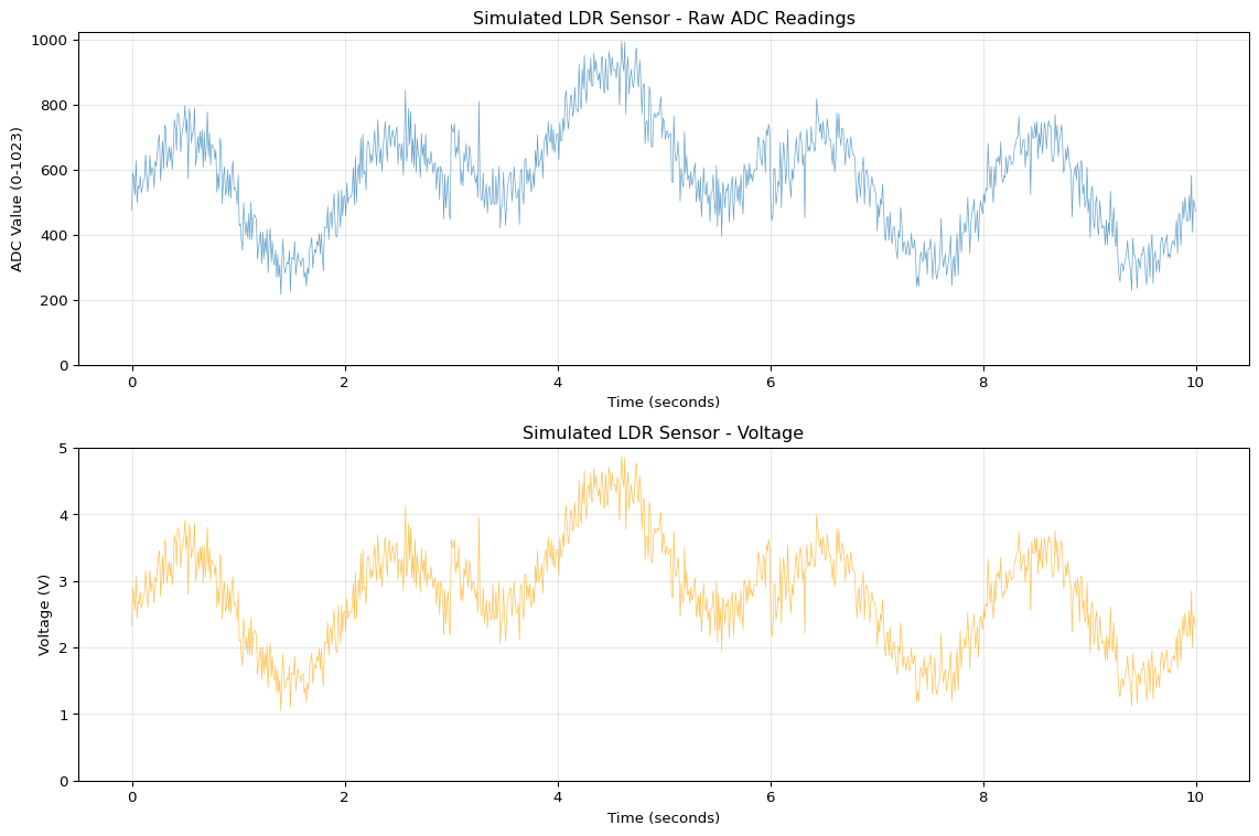
Generate realistic sensor data with noise characteristics similar to real ADC readings from Arduino sensors.

import numpy as np
import matplotlib.pyplot as plt

def simulate_ldr_data(duration_sec=10, sample_rate=100, noise_level=0.05):
    """
    Simulate Light Dependent Resistor (LDR) readings with realistic noise.

    Args:
        duration_sec: Duration in seconds
        sample_rate: Samples per second (Hz)
        noise_level: Noise amplitude (0-1)

    Returns:
        time, raw_values (ADC 0-1023), voltage (0-5V)
    """
    num_samples = duration_sec * sample_rate
    time = np.linspace(0, duration_sec, num_samples)

    # Simulate varying light conditions (sinusoidal + step changes)
    base_signal = 512 + 200 * np.sin(2 * np.pi * 0.5 * time)  # Slow oscillation

    # Add step changes (simulating light turning on/off)
    step_changes = np.where((time > 3) & (time < 6), 200, 0)
    base_signal += step_changes

    # Add realistic noise (Gaussian + occasional spikes)
    gaussian_noise = np.random.normal(0, noise_level * 1023, num_samples)
    spike_mask = np.random.random(num_samples) < 0.01  # 1% spike probability
    spikes = spike_mask * np.random.choice([-200, 200], num_samples)

    raw_values = base_signal + gaussian_noise + spikes
    raw_values = np.clip(raw_values, 0, 1023)  # ADC limits

    # Convert to voltage
    voltage = raw_values * (5.0 / 1023.0)

    return time, raw_values.astype(int), voltage

# Generate simulated sensor data
time, raw_adc, voltage = simulate_ldr_data(duration_sec=10, sample_rate=100, noise_level=0.05)

# Visualize
fig, (ax1, ax2) = plt.subplots(2, 1, figsize=(12, 8))

ax1.plot(time, raw_adc, linewidth=0.5, alpha=0.7)
ax1.set_xlabel('Time (seconds)')
ax1.set_ylabel('ADC Value (0-1023)')
ax1.set_title('Simulated LDR Sensor - Raw ADC Readings')
ax1.grid(alpha=0.3)
ax1.set_ylim(0, 1023)

ax2.plot(time, voltage, linewidth=0.5, alpha=0.7, color='orange')
ax2.set_xlabel('Time (seconds)')
ax2.set_ylabel('Voltage (V)')
ax2.set_title('Simulated LDR Sensor - Voltage')
ax2.grid(alpha=0.3)
ax2.set_ylim(0, 5)

plt.tight_layout()
plt.show()

print(f"Generated {len(raw_adc)} samples over {time[-1]:.1f} seconds")
print(f"Sample rate: {len(raw_adc) / time[-1]:.0f} Hz")
print(f"ADC range: {raw_adc.min()} - {raw_adc.max()}")
print(f"Voltage range: {voltage.min():.2f}V - {voltage.max():.2f}V")
print(f"Mean ADC value: {raw_adc.mean():.1f}")
print(f"Noise spikes detected: {np.sum(np.abs(np.diff(raw_adc)) > 100)}")

Generated 1000 samples over 10.0 seconds
Sample rate: 100 Hz
ADC range: 216 - 995
Voltage range: 1.06V - 4.86V
Mean ADC value: 568.6
Noise spikes detected: 169

Key Insight: Real sensor data contains both Gaussian noise (from electrical interference) and occasional spikes (from EMI, loose connections). Filtering is essential before using data for ML training.

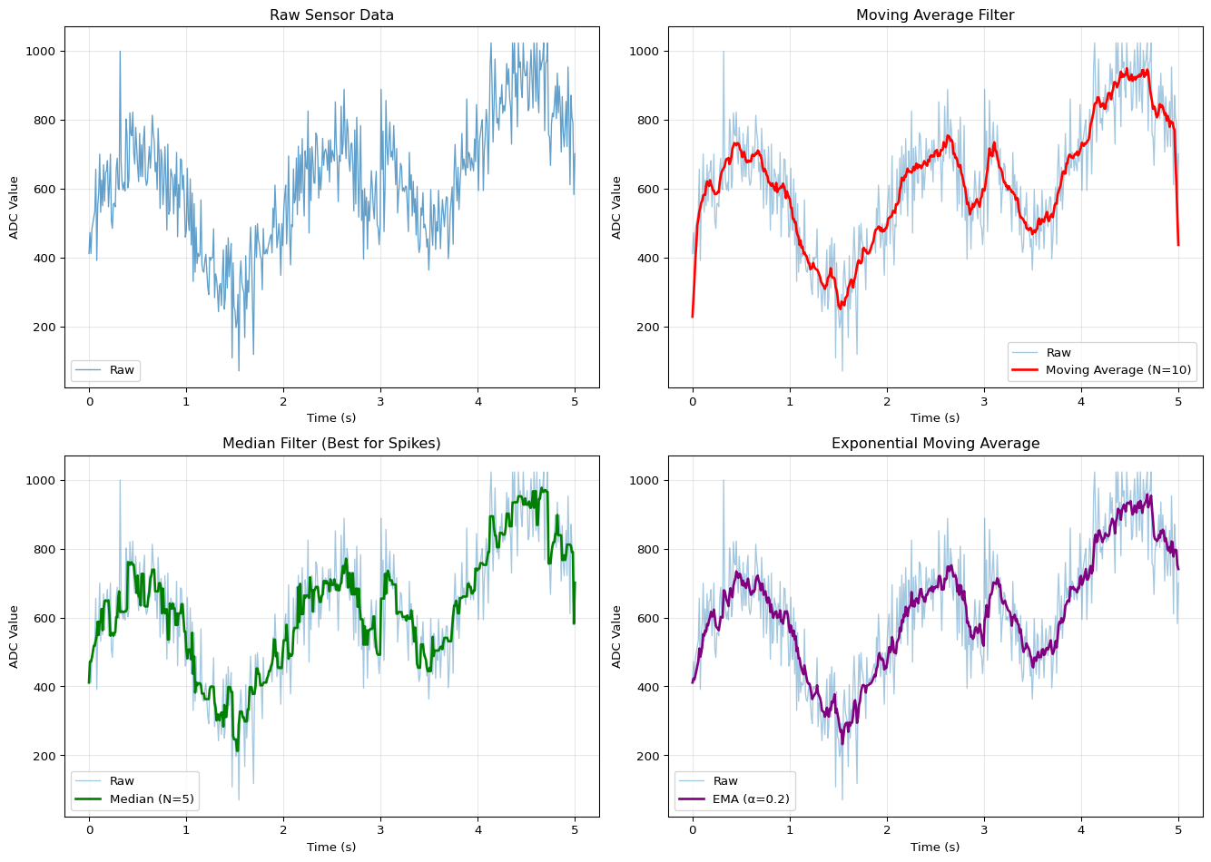
Moving Average Filter Implementation

Implement and compare different filtering techniques for noise reduction in sensor data.

def moving_average_filter(data, window_size=5):
    """Simple moving average filter using convolution."""
    kernel = np.ones(window_size) / window_size
    return np.convolve(data, kernel, mode='same')

def median_filter(data, window_size=5):
    """Median filter for spike rejection."""
    filtered = np.copy(data)
    half_window = window_size // 2

    for i in range(half_window, len(data) - half_window):
        window = data[i - half_window : i + half_window + 1]
        filtered[i] = np.median(window)

    return filtered

def exponential_moving_average(data, alpha=0.2):
    """Exponential moving average (EMA) for real-time filtering."""
    filtered = np.zeros_like(data)
    filtered[0] = data[0]

    for i in range(1, len(data)):
        filtered[i] = alpha * data[i] + (1 - alpha) * filtered[i-1]

    return filtered

# Generate noisy sensor data
time, raw_adc, voltage = simulate_ldr_data(duration_sec=5, sample_rate=100, noise_level=0.08)

# Apply different filters
ma_filtered = moving_average_filter(raw_adc, window_size=10)
median_filtered = median_filter(raw_adc, window_size=5)
ema_filtered = exponential_moving_average(raw_adc, alpha=0.2)

# Visualize comparison
fig, axes = plt.subplots(2, 2, figsize=(14, 10))

axes[0, 0].plot(time, raw_adc, linewidth=1, alpha=0.7, label='Raw')
axes[0, 0].set_title('Raw Sensor Data')
axes[0, 0].set_xlabel('Time (s)')
axes[0, 0].set_ylabel('ADC Value')
axes[0, 0].grid(alpha=0.3)
axes[0, 0].legend()

axes[0, 1].plot(time, raw_adc, linewidth=1, alpha=0.4, label='Raw')
axes[0, 1].plot(time, ma_filtered, linewidth=2, label='Moving Average (N=10)', color='red')
axes[0, 1].set_title('Moving Average Filter')
axes[0, 1].set_xlabel('Time (s)')
axes[0, 1].set_ylabel('ADC Value')
axes[0, 1].grid(alpha=0.3)
axes[0, 1].legend()

axes[1, 0].plot(time, raw_adc, linewidth=1, alpha=0.4, label='Raw')
axes[1, 0].plot(time, median_filtered, linewidth=2, label='Median (N=5)', color='green')
axes[1, 0].set_title('Median Filter (Best for Spikes)')
axes[1, 0].set_xlabel('Time (s)')
axes[1, 0].set_ylabel('ADC Value')
axes[1, 0].grid(alpha=0.3)
axes[1, 0].legend()

axes[1, 1].plot(time, raw_adc, linewidth=1, alpha=0.4, label='Raw')
axes[1, 1].plot(time, ema_filtered, linewidth=2, label='EMA (α=0.2)', color='purple')
axes[1, 1].set_title('Exponential Moving Average')
axes[1, 1].set_xlabel('Time (s)')
axes[1, 1].set_ylabel('ADC Value')
axes[1, 1].grid(alpha=0.3)
axes[1, 1].legend()

plt.tight_layout()
plt.show()

# Calculate noise reduction metrics
def calculate_snr(signal, filtered):
    """Calculate Signal-to-Noise Ratio improvement."""
    noise = signal - filtered
    signal_power = np.mean(filtered ** 2)
    noise_power = np.mean(noise ** 2)
    snr_db = 10 * np.log10(signal_power / noise_power) if noise_power > 0 else float('inf')
    return snr_db

print("=== Filter Performance Comparison ===\n")
print(f"Moving Average SNR: {calculate_snr(raw_adc, ma_filtered):.1f} dB")
print(f"Median Filter SNR:  {calculate_snr(raw_adc, median_filtered):.1f} dB")
print(f"EMA SNR:            {calculate_snr(raw_adc, ema_filtered):.1f} dB")

# Show spike rejection capability
num_spikes_raw = np.sum(np.abs(np.diff(raw_adc)) > 100)
num_spikes_ma = np.sum(np.abs(np.diff(ma_filtered)) > 100)
num_spikes_median = np.sum(np.abs(np.diff(median_filtered)) > 100)

print(f"\n=== Spike Rejection ===\n")
print(f"Raw data spikes:      {num_spikes_raw}")
print(f"Moving Average:       {num_spikes_ma} ({(1 - num_spikes_ma/num_spikes_raw)*100:.1f}% reduction)")
print(f"Median Filter:        {num_spikes_median} ({(1 - num_spikes_median/num_spikes_raw)*100:.1f}% reduction)")
print("\nRecommendation: Use Median filter for spike rejection, Moving Average for general smoothing")

=== Filter Performance Comparison ===

Moving Average SNR: 18.1 dB
Median Filter SNR:  18.6 dB
EMA SNR:            18.9 dB

=== Spike Rejection ===

Raw data spikes:      197
Moving Average:       0 (100.0% reduction)
Median Filter:        13 (93.4% reduction)

Recommendation: Use Median filter for spike rejection, Moving Average for general smoothing

Key Insight: Median filters excel at removing spikes while preserving signal edges. Moving average filters smooth noise but can blur rapid changes. Choose based on your application needs.

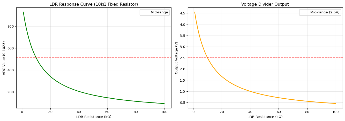
Voltage Divider Calculator

Calculate resistor values for LDR and other resistive sensor circuits.

def voltage_divider(v_in, r1, r2):
    """Calculate output voltage of voltage divider."""
    return v_in * (r2 / (r1 + r2))

def calculate_adc_value(v_out, v_ref=5.0, bits=10):
    """Convert voltage to ADC value."""
    max_value = (2 ** bits) - 1
    return int((v_out / v_ref) * max_value)

def design_ldr_circuit(r_ldr_range, v_in=5.0, target_mid=512):
    """
    Design optimal fixed resistor for LDR voltage divider.

    Args:
        r_ldr_range: Tuple of (min_resistance, max_resistance) in ohms
        v_in: Supply voltage
        target_mid: Desired ADC value at mid-range

    Returns:
        Optimal fixed resistor value
    """
    r_min, r_max = r_ldr_range
    r_mid = np.sqrt(r_min * r_max)  # Geometric mean

    # For target_mid ADC value, solve voltage divider
    v_target = (target_mid / 1023) * v_in
    r_fixed = r_mid * (v_in - v_target) / v_target

    return r_fixed

# Example: LDR with range 1kΩ (bright) to 100kΩ (dark)
r_ldr_bright = 1000    # 1kΩ in bright light
r_ldr_dark = 100000    # 100kΩ in darkness
r_fixed = design_ldr_circuit((r_ldr_bright, r_ldr_dark))

print("=== LDR Voltage Divider Design ===\n")
print(f"LDR range: {r_ldr_bright/1000:.1f}kΩ (bright) to {r_ldr_dark/1000:.1f}kΩ (dark)")
print(f"Recommended fixed resistor: {r_fixed/1000:.1f}kΩ")
print(f"Standard value: 10kΩ\n")

# Simulate ADC readings across light levels
r_ldr_values = np.linspace(r_ldr_bright, r_ldr_dark, 100)
r_fixed_actual = 10000  # 10kΩ standard resistor

adc_values = []
voltages = []

for r_ldr in r_ldr_values:
    v_out = voltage_divider(5.0, r_ldr, r_fixed_actual)
    adc = calculate_adc_value(v_out)
    voltages.append(v_out)
    adc_values.append(adc)

# Visualize response curve
fig, (ax1, ax2) = plt.subplots(1, 2, figsize=(14, 5))

ax1.plot(r_ldr_values / 1000, adc_values, linewidth=2, color='green')
ax1.set_xlabel('LDR Resistance (kΩ)')
ax1.set_ylabel('ADC Value (0-1023)')
ax1.set_title('LDR Response Curve (10kΩ Fixed Resistor)')
ax1.grid(alpha=0.3)
ax1.axhline(512, color='red', linestyle='--', alpha=0.5, label='Mid-range')
ax1.legend()

ax2.plot(r_ldr_values / 1000, voltages, linewidth=2, color='orange')
ax2.set_xlabel('LDR Resistance (kΩ)')
ax2.set_ylabel('Output Voltage (V)')
ax2.set_title('Voltage Divider Output')
ax2.grid(alpha=0.3)
ax2.axhline(2.5, color='red', linestyle='--', alpha=0.5, label='Mid-range (2.5V)')
ax2.legend()

plt.tight_layout()
plt.show()

# Calculate useful ranges
sensitive_range = np.where((np.array(adc_values) > 200) & (np.array(adc_values) < 823))[0]
r_ldr_sensitive = r_ldr_values[sensitive_range]

print(f"=== Circuit Performance ===\n")
print(f"Bright light (1kΩ):  ADC = {adc_values[0]}, Voltage = {voltages[0]:.2f}V")
print(f"Mid-range (10kΩ):    ADC = {adc_values[50]}, Voltage = {voltages[50]:.2f}V")
print(f"Darkness (100kΩ):    ADC = {adc_values[-1]}, Voltage = {voltages[-1]:.2f}V")
print(f"\nSensitive range: {r_ldr_sensitive[0]/1000:.1f}kΩ to {r_ldr_sensitive[-1]/1000:.1f}kΩ")
print(f"ADC resolution in sensitive range: {len(sensitive_range)} distinct values")

=== LDR Voltage Divider Design ===

LDR range: 1.0kΩ (bright) to 100.0kΩ (dark)
Recommended fixed resistor: 10.0kΩ
Standard value: 10kΩ

=== Circuit Performance ===

Bright light (1kΩ):  ADC = 929, Voltage = 4.55V
Mid-range (10kΩ):    ADC = 167, Voltage = 0.82V
Darkness (100kΩ):    ADC = 93, Voltage = 0.45V

Sensitive range: 3.0kΩ to 40.0kΩ
ADC resolution in sensitive range: 38 distinct values

Key Insight: Choose the fixed resistor value near the geometric mean of your sensor’s resistance range for maximum sensitivity. Standard 10kΩ resistors work well for most LDRs.

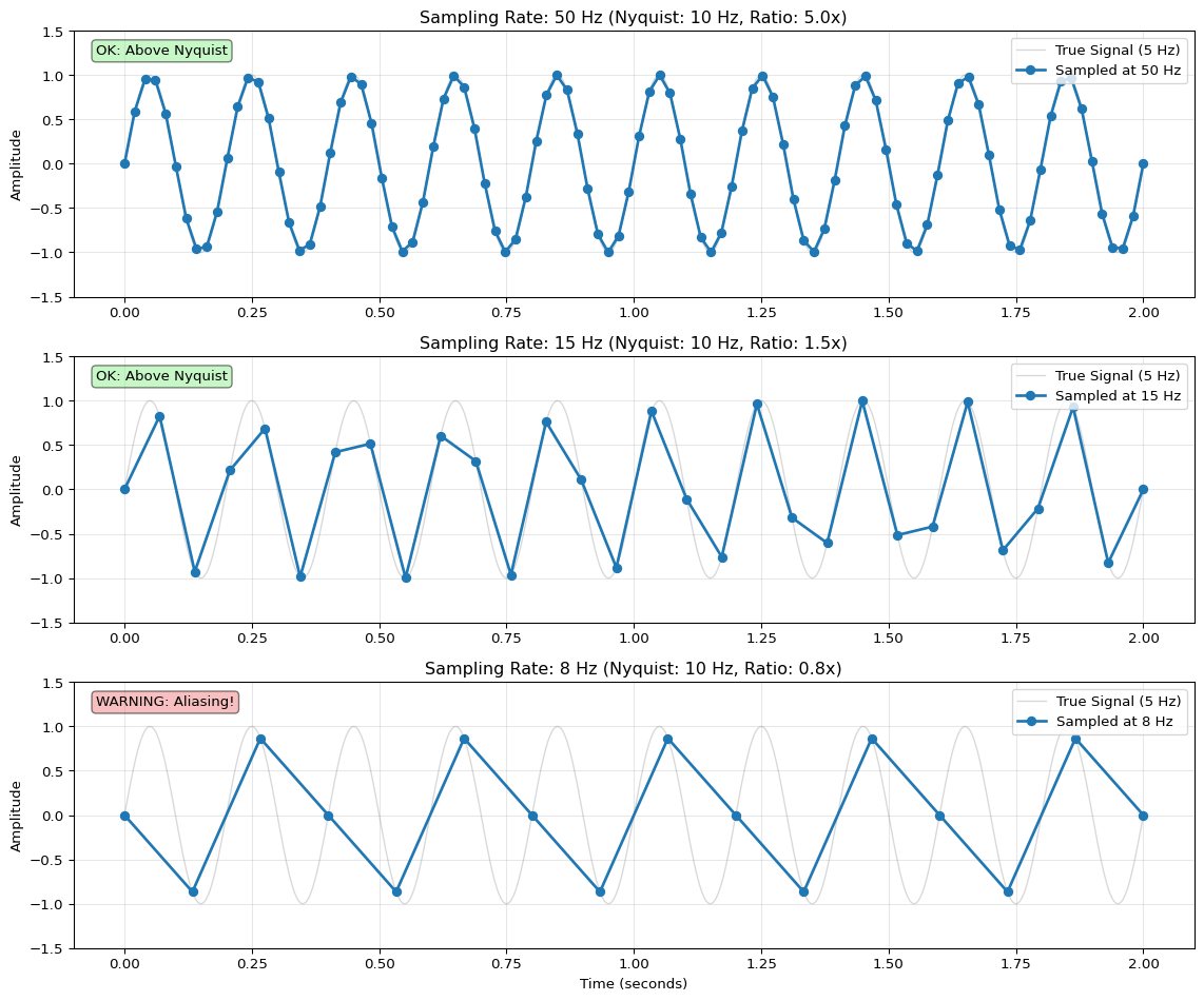
Sampling Rate Analysis

Understand the relationship between sampling rate, signal frequency, and aliasing (Nyquist theorem).

def generate_signal(freq, duration, sample_rate):
    """Generate sinusoidal signal."""
    t = np.linspace(0, duration, int(duration * sample_rate))
    signal = np.sin(2 * np.pi * freq * t)
    return t, signal

# Demonstrate Nyquist theorem and aliasing
signal_freq = 5  # 5 Hz signal
duration = 2

# Different sampling rates
sample_rates = [50, 15, 8]  # Adequate, Marginal, Aliased

fig, axes = plt.subplots(len(sample_rates), 1, figsize=(12, 10))

# Generate ground truth (high sample rate)
t_truth, signal_truth = generate_signal(signal_freq, duration, 1000)

for idx, fs in enumerate(sample_rates):
    t_sampled, signal_sampled = generate_signal(signal_freq, duration, fs)

    axes[idx].plot(t_truth, signal_truth, 'gray', alpha=0.3, linewidth=1, label='True Signal (5 Hz)')
    axes[idx].plot(t_sampled, signal_sampled, 'o-', linewidth=2, markersize=6, label=f'Sampled at {fs} Hz')
    axes[idx].set_ylabel('Amplitude')
    axes[idx].set_title(f'Sampling Rate: {fs} Hz (Nyquist: {signal_freq * 2} Hz, Ratio: {fs / (2*signal_freq):.1f}x)')
    axes[idx].grid(alpha=0.3)
    axes[idx].legend()
    axes[idx].set_ylim(-1.5, 1.5)

    # Add Nyquist indicator
    if fs >= 2 * signal_freq:
        axes[idx].text(0.02, 0.95, 'OK: Above Nyquist', transform=axes[idx].transAxes,
                      fontsize=10, verticalalignment='top',
                      bbox=dict(boxstyle='round', facecolor='lightgreen', alpha=0.5))
    else:
        axes[idx].text(0.02, 0.95, 'WARNING: Aliasing!', transform=axes[idx].transAxes,
                      fontsize=10, verticalalignment='top',
                      bbox=dict(boxstyle='round', facecolor='lightcoral', alpha=0.5))

axes[-1].set_xlabel('Time (seconds)')
plt.tight_layout()
plt.show()

# Common sensor sampling recommendations
print("=== Recommended Sampling Rates for Edge ML ===\n")

sensors = [
    ("Temperature (DHT11)", "0.1 Hz", "Slow thermal changes"),
    ("Light (LDR)", "10 Hz", "Human perception ~60 Hz, but 10 Hz sufficient"),
    ("Accelerometer (Gesture)", "50-100 Hz", "Human motion ~20 Hz, 2-5x Nyquist"),
    ("Microphone (Audio)", "16 kHz", "Human speech 300-3400 Hz, 4x Nyquist"),
    ("EMG (Muscle)", "500-1000 Hz", "EMG signals 20-500 Hz, 2x Nyquist"),
]

for sensor, rate, reason in sensors:
    print(f"{sensor:30s}: {rate:10s} - {reason}")

print("\nKey Rule: Sample at 2-5× the highest frequency component (Nyquist theorem)")
print("Higher rates = better fidelity but more memory and power consumption")

=== Recommended Sampling Rates for Edge ML ===

Temperature (DHT11)           : 0.1 Hz     - Slow thermal changes
Light (LDR)                   : 10 Hz      - Human perception ~60 Hz, but 10 Hz sufficient
Accelerometer (Gesture)       : 50-100 Hz  - Human motion ~20 Hz, 2-5x Nyquist
Microphone (Audio)            : 16 kHz     - Human speech 300-3400 Hz, 4x Nyquist
EMG (Muscle)                  : 500-1000 Hz - EMG signals 20-500 Hz, 2x Nyquist

Key Rule: Sample at 2-5× the highest frequency component (Nyquist theorem)
Higher rates = better fidelity but more memory and power consumption

Key Insight: The Nyquist theorem requires sampling at least 2× the signal frequency. For ML applications, use 2-5× Nyquist for safety. Balance data quality with memory/power constraints.

Self-Assessment Checkpoints

Test your understanding before proceeding to the exercises.

Question 1: Calculate the ADC voltage reading for an analog sensor that outputs 512 on a 10-bit Arduino ADC with 5V reference.

Answer: Voltage = (ADC_Value × V_ref) / (2^resolution - 1) = (512 × 5.0) / (1023) = 2560 / 1023 = 2.50 volts. The 10-bit ADC provides 1024 discrete levels (0-1023), with each step representing 5V / 1024 = 4.88 mV resolution. A reading of 512 (exactly half of 1023) corresponds to approximately half the reference voltage (2.5V).

Question 2: Why do you need a voltage divider circuit for resistive sensors like LDRs and thermistors?

Answer: The Arduino ADC measures voltage, not resistance. Resistive sensors change resistance based on physical conditions (light, temperature), but connecting an LDR directly between 5V and GND doesn’t create a measurable voltage at the analog pin. A voltage divider circuit (LDR + fixed resistor) converts resistance changes into voltage changes: V_out = 5V × (R_fixed / (R_sensor + R_fixed)). As the sensor resistance changes, the voltage divider output changes proportionally, which the ADC can measure. Without the fixed resistor, the ADC reads either 0V or 5V with no intermediate values.

Question 3: Your analog sensor readings jump randomly between 200 and 800 even when the sensor is stable. What’s wrong and how do you fix it?

Answer: Electrical noise, EMI, or loose wiring causes these spikes. Solutions: (1) Moving average filter: Average the last 5-10 readings to smooth noise: smoothed = (sum of last N readings) / N, (2) Median filter: Take the median of 5 readings to reject outliers (more robust than average), (3) Hardware fixes: Add a 0.1μF capacitor between analog pin and GND to filter high-frequency noise, ensure solid wiring connections, keep sensor wires short and away from power lines, (4) Software debouncing: Ignore readings that change more than a threshold from previous values. Always filter raw sensor data before feeding to ML models.

Question 4: Why is consistent sampling rate critical for ML training data collection?

Answer: ML models trained on time-series data (audio, motion, EMG) learn temporal patterns based on fixed time intervals. If training uses 100 Hz sampling (10ms intervals) but deployment uses variable delays (8-15ms), the model receives distorted patterns and fails. Example: A gesture recognition model learns that “wave motion” has 3 peaks in 50 samples. If deployment samples irregularly, those peaks might appear in 40 or 60 samples, confusing the model. Solutions: Use fixed delay(10) for 100 Hz, or better yet, use timer interrupts for precise timing. Document and match the exact sampling rate in both training and deployment.

Question 5: When should you use digital sensors (I2C/SPI) versus analog sensors for edge ML applications?

Answer: Use digital sensors when: (1) You need pre-calibrated, accurate values (DHT11 temperature, MPU6050 accelerometer), (2) Multiple sensors on one bus (I2C supports multiple addresses), (3) Long wires (digital signals are noise-resistant), (4) Convenience matters (no ADC math, no calibration curves). Use analog sensors when: (1) Cost is critical (LDRs are $0.10, digital light sensors are $2+), (2) You need custom behavior or unusual sensors, (3) Simple applications (1-2 sensors), (4) Learning/prototyping (easier to understand). For production edge ML: prefer digital sensors for reliability and ease of integration; use analog for cost-sensitive applications.

Interactive Notebook

The notebook below contains runnable code for all Level 1 activities.

LAB08: Arduino Sensors and Signal Acquisition

Learning Objectives: - Understand how sensors convert physical phenomena to electrical signals - Learn ADC (Analog-to-Digital Conversion) fundamentals - Apply the Nyquist sampling theorem for proper data acquisition - Implement digital filters to remove noise from sensor readings - Build a multi-sensor data logging system

Three-Tier Approach: - Level 1 (This Notebook): Simulate sensors and learn signal processing - Level 2 (Wokwi): Test code in browser-based Arduino simulator - Level 3 (Device): Deploy on real Arduino with physical sensors

1. Setup

2. Understanding Sensors: From Physics to Voltage

How Sensors Work

Sensors are transducers - they convert one form of energy into another. For microcontrollers, we need to convert physical phenomena into electrical signals.

Physical Phenomenon	Sensor Type	Conversion Principle
Light	Photoresistor (LDR)	Resistance changes with light intensity
Temperature	Thermistor	Resistance changes with temperature
Force/Pressure	Piezoelectric	Mechanical stress generates voltage
Motion	Accelerometer	Capacitance changes with displacement

The Thermistor: A Worked Example

A thermistor’s resistance follows the Steinhart-Hart equation:

\(\frac{1}{T} = A + B \cdot \ln(R) + C \cdot (\ln(R))^3\)

Where: - \(T\) = Temperature in Kelvin - \(R\) = Resistance in Ohms - \(A, B, C\) = Calibration coefficients (from datasheet)

For a typical NTC thermistor (10kΩ at 25°C), a simpler approximation works:

\(R = R_0 \cdot e^{\beta(\frac{1}{T} - \frac{1}{T_0})}\)

Where \(\beta \approx 3950\) for common thermistors.

3. Analog-to-Digital Conversion (ADC)

The Problem: Microcontrollers Only Understand Digital

Physical sensors produce continuous analog signals, but microcontrollers process discrete digital values. The ADC bridges this gap.

ADC Fundamentals

An ADC converts a continuous voltage range into discrete digital steps:

\(\text{Digital Value} = \text{round}\left(\frac{V_{in}}{V_{ref}} \times (2^n - 1)\right)\)

Where: - \(V_{in}\) = Input voltage from sensor - \(V_{ref}\) = Reference voltage (5V for Arduino Uno) - \(n\) = ADC resolution in bits (10 bits for Arduino Uno)

Arduino Uno ADC Specifications

Parameter	Value
Resolution	10 bits (0-1023)
Reference Voltage	5V (default)
Voltage per Step	5V / 1024 = 4.88mV
Conversion Time	~100μs
Max Sample Rate	~10,000 samples/sec

Quantization Error

The ADC introduces quantization error because continuous values are rounded to discrete steps:

\(\text{Quantization Error} = \pm \frac{\text{LSB}}{2} = \pm \frac{V_{ref}}{2^{n+1}}\)

For Arduino: \(\pm 2.44\text{mV}\)

💡 Alternative Approaches

Option A: Step-wise ADC (Current approach) - Pros: Matches real hardware behavior, intuitive visualization - Cons: Always rounds (introduces quantization error)

Option B: Dithering ADC - Pros: Reduces quantization noise through intentional randomization - Cons: Slightly more complex, may confuse beginners - Code modification: Add + np.random.uniform(-0.5, 0.5) before rounding

Option C: Oversampling ADC - Pros: Achieves higher effective resolution (e.g., 4× sampling → +1 bit) - Cons: Requires averaging, slower sampling rate - Code modification: Sample 4 times, average, then convert

When to use each: - Use Option A for learning and matching Arduino exactly - Use Option B for audio applications where quantization noise is audible - Use Option C when you need 11-bit precision from 10-bit ADC (medical sensors)

4. The Nyquist Sampling Theorem

Why Sampling Rate Matters

When we sample a continuous signal, we must sample fast enough to capture all the information. The Nyquist-Shannon Sampling Theorem states:

\(f_s \geq 2 \cdot f_{max}\)

Where: - \(f_s\) = Sampling frequency (samples per second) - \(f_{max}\) = Highest frequency component in the signal

Aliasing: What Happens When You Sample Too Slowly

If you violate Nyquist, high frequencies “fold back” and appear as fake low frequencies - this is called aliasing.

Practical Guidelines for Sensor Sampling

Signal Type	Typical Frequency	Min Sample Rate	Recommended
Temperature	< 0.1 Hz	0.2 Hz	1 Hz
Human motion	0-10 Hz	20 Hz	50 Hz
Vibration	10-1000 Hz	2 kHz	5 kHz
Audio	20-20000 Hz	40 kHz	44.1 kHz

🔬 Try It Yourself

Modify the sampling parameters and observe the effects:

Parameter	Current	Try These	Expected Effect
f_signal	5 Hz	1, 10, 20 Hz	Higher freq requires higher sample rate
fs_good	50 Hz	20, 100, 200 Hz	More samples = smoother reconstruction
fs_alias	6 Hz	4, 8, 9 Hz	Different aliased frequencies appear

Experiment 1: Change f_signal = 10 and keep fs_alias = 6. What frequency do you perceive?

Answer: You’ll see apparent frequency of |10 - 6| = 4 Hz (aliasing)

Experiment 2: Set fs_good = 10 (exactly Nyquist). What happens?

Answer: Reconstruction is theoretically possible but phase-sensitive (risky in practice)

💡 Alternative Approaches: Digital Filters

Option A: Exponential Filter (Current approach) - Pros: Memory-efficient (1 value), fast, simple - Cons: Fixed time constant, phase lag - Formula: y[n] = α·x[n] + (1-α)·y[n-1]

Option B: Moving Average Filter - Pros: Symmetric (no phase lag), intuitive - Cons: Requires buffer of N samples (more memory) - Code modification: Replace ExponentialFilter with MovingAverageFilter(N=10)

Option C: Median Filter - Pros: Excellent for removing spikes/outliers (salt-and-pepper noise) - Cons: Non-linear (harder to analyze), requires sorting - Code: filtered = np.median(buffer[-N:])

Option D: Kalman Filter - Pros: Optimal for linear systems with known noise model - Cons: Complex, requires tuning Q and R matrices - Use case: High-precision sensor fusion (IMU)

When to use each: - Use Option A (exponential) for MCUs with limited RAM - Use Option B (moving average) when you need linear phase response - Use Option C (median) for outlier rejection (e.g., ultrasonic sensors) - Use Option D (Kalman) for professional applications with noise characterization

🔬 Try It Yourself: Filter Parameters

Experiment with filter parameters to see their effect:

Parameter	Current	Try These	Expected Effect
alpha (EMA)	0.2	0.05, 0.5, 0.9	Lower = smoother but slower response
window_size (MA)	10	5, 20, 50	Larger = smoother but more lag

Experiment 1: Step Response

# Create step function
signal_step = np.concatenate([np.ones(50)*10, np.ones(50)*20])
# Apply filters with different alpha
for alpha in [0.1, 0.3, 0.7]:
    filt = ExponentialFilter(alpha)
    output = [filt.update(x) for x in signal_step]
    plt.plot(output, label=f'α={alpha}')

What to observe: Lower α → slower rise time (more smoothing)

Experiment 2: Frequency Response

# Sweep through frequencies
for freq in [0.1, 1, 10]:  # Hz
    test_signal = np.sin(2*np.pi*freq*t)
    # Apply filter and compare amplitude

What to observe: High frequencies get attenuated (low-pass behavior)

5. Digital Filtering: Removing Noise

Why Filter?

Real sensor signals contain noise from various sources: - Electrical interference (50/60 Hz powerline) - Thermal noise in electronics - Mechanical vibration - Quantization noise from ADC

Moving Average Filter

The simplest filter averages the last \(N\) samples:

\(y[n] = \frac{1}{N} \sum_{i=0}^{N-1} x[n-i]\)

Trade-off: Larger \(N\) = smoother output but slower response to real changes.

Exponential Moving Average (EMA)

More memory-efficient and gives more weight to recent samples:

\(y[n] = \alpha \cdot x[n] + (1-\alpha) \cdot y[n-1]\)

Where \(\alpha\) (0 to 1) controls smoothing: - \(\alpha = 1\): No filtering (output = input) - \(\alpha = 0.1\): Heavy smoothing - \(\alpha = 0.5\): Moderate smoothing

Memory: Only needs to store ONE previous value!

6. Complete Sensor Simulation

Now let’s put it all together with a realistic sensor simulation that includes: - Physical sensor model - ADC conversion - Noise - Filtering

⚠️ Common Issues and Debugging

If ADC readings are unstable/noisy: - Check: Are you using floating wires? → Solution: Twist/shield wires, keep them short - Check: Is sensor powered from same rail as MCU? → Solution: Use separate regulated supply - Check: Missing pull-down resistor? → Solution: Add 10kΩ to ground on analog input

If filter output has unexpected lag: - Check: Is α too small? → Solution: Increase α (but increases noise) - Check: Is moving average window too large? → Solution: Reduce N - Formula: Time constant τ ≈ 1/(α·fs), where fs = sampling rate

If seeing aliasing artifacts: - Check: Is sampling rate at least 2× highest frequency? → Solution: Increase sample rate or add analog anti-aliasing filter - Hardware fix: Add RC low-pass filter before ADC (R=1kΩ, C=0.1µF for ~1.6kHz cutoff)

If readings are clipping at 0 or 1023: - Check: Is sensor output exceeding 0-5V range? → Solution: Use voltage divider - Check: Is there DC offset? → Solution: AC couple with capacitor - Diagnostic: Print raw ADC values to verify range

Arduino-specific issues: - analogRead() takes ~100µs → Max sample rate ~10kHz (not 16MHz!) - ADC reference affects accuracy: use analogReference(EXTERNAL) for precision - First ADC reading after switching channels may be inaccurate (throw away first sample)

7. Arduino Code Reference

Here’s the equivalent Arduino code for reading sensors with filtering:

8. Checkpoint Questions

1. ADC Resolution: An Arduino Uno has 10-bit ADC. What is the smallest voltage change it can detect?

2. Nyquist Theorem: You want to measure a motor’s vibration at up to 500 Hz. What’s the minimum sampling rate?

3. Filter Trade-offs: Why can’t we just use a very large moving average window (e.g., N=1000)?

4. Memory Efficiency: Why is the exponential filter preferred on microcontrollers over moving average?

5. Practical Application: A temperature sensor updates slowly (< 0.1 Hz) but has high-frequency noise. Design a filtering strategy.

9. Next Steps

Level 2: Wokwi Simulator

Test your Arduino code in the browser: LAB08 Wokwi Simulation

Level 3: Physical Hardware

• Connect real sensors to Arduino
• Verify filter performance with actual noise
• Log data to SD card or send via serial

See Chapter 8 in the textbook for circuit diagrams and advanced topics.

10. Multi-Sensor Simulation: IMU (Accelerometer + Gyroscope)

Real-world edge devices often combine multiple sensors. Let’s simulate a 6-axis IMU (Inertial Measurement Unit) commonly used in: - Wearable fitness trackers - Drone stabilization - Gesture recognition - Fall detection systems

IMU Physics

Accelerometer measures linear acceleration in 3 axes: \(\vec{a} = [a_x, a_y, a_z]\)

At rest: measures gravity (\(9.81 \text{ m/s}^2\)) in the down direction.

Gyroscope measures angular velocity (rotation rate): \(\vec{\omega} = [\omega_x, \omega_y, \omega_z]\)

Units: degrees/second or radians/second

11. Advanced Preprocessing: Sensor Calibration

Real sensors have systematic errors (bias) and scaling errors (gain). Calibration corrects these:

\(x_{\text{calibrated}} = \frac{x_{\text{raw}} - \text{bias}}{\text{gain}}\)

For accelerometers, we can calibrate using gravity as a known reference.

12. ML Feature Extraction from Sensor Data

For activity recognition and gesture detection, we extract statistical features from sensor windows.

13. Advanced Visualization: Real-Time Sensor Dashboard

Create an informative sensor dashboard showing multiple visualizations simultaneously.

14. Summary and Key Takeaways

What You Learned

1. Sensor Physics: How transducers convert physical signals to electrical (thermistor equation)
2. ADC Fundamentals: Quantization, resolution (4.88mV for Arduino), sampling rate
3. Nyquist Theorem: Must sample ≥2× highest frequency to avoid aliasing
4. Digital Filtering: Moving average, exponential filters for noise reduction
5. Multi-sensor Systems: IMU simulation with accelerometer + gyroscope
6. Calibration: Correcting bias and gain errors
7. Feature Extraction: Statistical features for ML classification
8. Data Visualization: Creating informative sensor dashboards

Edge Analytics Pipeline

[Sensor] → [ADC] → [Filter] → [Features] → [ML Model] → [Decision]

Ready for Hardware

All concepts in this notebook transfer directly to Arduino/ESP32: - Use analogRead() for ADC - Implement filters in C++ - Extract features in real-time - Deploy TinyML models

See LAB 8 Wokwi Simulation and Chapter 8 for hardware deployment!

Three-Tier Activities

Level 1: Notebook

Run the embedded notebook above. Key exercises:

1. Follow along with the code cells
2. Modify parameters and observe results
3. Complete the checkpoint questions

Level 2: Simulator

Arduino Multi-Sensor Simulator

Program real Arduino code in your browser using Wokwi:

• Multi-sensor data logging (analog + digital)
• Serial output and data visualization
• LED threshold indicators
• No hardware required!

Level 3: Device

Multi-sensor data logger

Visual Troubleshooting

Sensor Reading Problems

flowchart TD
    A[Bad sensor readings] --> B{Sensor type?}
    B -->|Analog ADC| C{Reading always 0 or 1023?}
    C -->|Yes| D[Check wiring:<br/>Need voltage divider?<br/>Correct analog pin?<br/>Ground OK?]
    C -->|Values but noisy| E[Add filtering:<br/>Moving average 5-10<br/>Median for spikes<br/>Hardware low-pass filter]
    B -->|Digital I2C/SPI| F{Communication OK?}
    F -->|No response| G[Check I2C address<br/>Scan for devices<br/>Pull-up resistors 4.7kΩ]
    F -->|Intermittent| H[Check connections:<br/>Loose wires?<br/>Cable too long?<br/>EMI interference?]
    B -->|Timing issues| I[Use millis timing:<br/>if millis - last >= interval<br/>Fixed sample rate]

    style A fill:#ff6b6b
    style D fill:#4ecdc4
    style E fill:#4ecdc4
    style G fill:#4ecdc4
    style H fill:#4ecdc4
    style I fill:#4ecdc4

Arduino Upload Failures

flowchart TD
    A[Upload fails] --> B{Port shown?}
    B -->|No| C[Check USB:<br/>Different cable<br/>Different port<br/>Restart IDE]
    B -->|Yes| D{Correct board?}
    D -->|No| E[Tools → Board<br/>Select Arduino Nano 33 BLE<br/>or your specific board]
    D -->|Yes| F{Error type?}
    F -->|Timeout| G[Press reset 2x quickly<br/>Enter bootloader<br/>Upload within 8s]
    F -->|Sketch too big| H[Reduce size:<br/>MicroMutableOpResolver<br/>Remove debug prints<br/>Smaller model]

    style A fill:#ff6b6b
    style C fill:#4ecdc4
    style E fill:#4ecdc4
    style G fill:#4ecdc4
    style H fill:#4ecdc4

For complete troubleshooting flowcharts, see:

• Sensor Reading Problems
• Arduino Upload Failures
• All Visual Troubleshooting Guides

Related Labs

Hardware Integration

• LAB05: Edge Deployment - Deploy ML models to Arduino
• LAB09: ESP32 Wireless - Add wireless connectivity to sensor nodes
• LAB10: EMG Biomedical - Advanced signal processing with sensors

Data Pipelines

• LAB12: Streaming - Stream sensor data to processing pipelines
• LAB13: Distributed Data - Store and query sensor readings

Related Resources

• Hardware Guide - Equipment needed for Level 3
• Troubleshooting - Common issues and solutions