LAB15: Energy Optimization

Power-Efficient Edge Computing

PDF Textbook Reference

For detailed theoretical foundations, mathematical proofs, and algorithm derivations, see Chapter 15: Energy-Aware Edge Computing and Optimization in the PDF textbook.

The PDF chapter includes: - Complete power consumption models for MCUs and peripherals - Detailed mathematical derivations of battery life calculations - In-depth DVFS (Dynamic Voltage Frequency Scaling) theory - Comprehensive duty cycle optimization algorithms - Theoretical analysis of early-exit networks and adaptive inference

Open In Colab

Download Notebook

Learning Objectives

By the end of this lab you should be able to:

• Estimate the energy consumption and battery life of an edge ML system from simple power models
• Measure real power and energy on development boards using USB meters or current sensors
• Apply quantization, duty cycling, and early-exit models to trade accuracy for energy savings
• Identify whether radio, CPU, sensors, or memory dominate the energy budget in a given design

Theory Summary

The Energy Equation

For battery-powered edge devices, energy is the ultimate constraint. A model achieving 99% accuracy but draining the battery in 2 hours is useless for wearables that need to last a week.

Three fundamental equations govern battery life:

• Power (mW) = Voltage (V) × Current (mA)
• Energy (mWh) = Power (mW) × Time (hours)
• Battery Life (hours) = Capacity (mAh) / Average Current (mA)

Example: A 2500 mAh LiPo battery at 3.7V contains 2500 × 3.7 = 9,250 mWh of energy. If your device draws an average of 10 mA, battery life is 2500 / 10 = 250 hours (10.4 days).

Where Power Goes: Component Breakdown

The biggest surprise for edge ML newcomers: the radio often dominates the power budget, not ML inference.

Typical power consumption for IoT devices: - WiFi transmission: 200-400 mW (dominates!) - BLE transmission: 10-50 mW (10× less than WiFi) - CPU active (inference): 50-200 mW - CPU idle: 1-10 mW - Deep sleep: 0.01-0.1 mW (1000× less than active) - Sensors: 0.1-10 mW - Display: 50-200 mW

A single WiFi transmission burst can use more energy than 1,000 ML inferences. Therefore, reducing transmission frequency by 2× often saves more energy than halving inference time.

Quantization and Energy Efficiency

INT8 inference is 10-18× more energy-efficient than FP32:

1. Simpler operations: INT8 multiply-accumulate uses less energy than floating-point
2. Smaller memory footprint: 4× smaller model = 4× less memory traffic
3. Faster memory access: Smaller data fits in fast, low-power SRAM instead of expensive DRAM

Memory access energy costs (approximate): - DRAM read: 640 pJ (picojoules) - SRAM read: 5 pJ (128× less!) - INT8 MAC: 0.2 pJ - FP32 MAC: 3.7 pJ

This is why quantization (from LAB03) is critical not just for speed, but for battery life.

Duty Cycling: The Ultimate Energy Saver

Spending 99% of time in deep sleep can extend battery life from hours to months.

Example calculation: - Deep sleep: 0.01 mA (99% of time) - Active + inference: 80 mA (1% of time) - Average current: (0.01 × 0.99) + (80 × 0.01) = 0.0099 + 0.8 = 0.81 mA - Battery life with 2500 mAh: 2500 / 0.81 = 3,086 hours (128 days)

Without sleep (constant 80 mA): 2500 / 80 = 31 hours (1.3 days). Sleep modes provide a 100× improvement!

Key Concepts at a Glance

Core Concepts

• Average Current is Key: Battery life = Capacity / Average current; reduce average through duty cycling
• Radio Dominates: WiFi uses 200-400 mW; a single transmission = 1000 inferences worth of energy
• Quantization Saves Energy: INT8 is 10-18× more efficient than FP32 due to simpler ops and less memory traffic
• Deep Sleep is Essential: ESP32 deep sleep uses 0.01 mA vs 80 mA active (8000× reduction!)
• Energy per Operation: DRAM read (640 pJ) >> FP32 MAC (3.7 pJ) >> INT8 MAC (0.2 pJ)
• Duty Cycle Formula: Average = (I_sleep × d_sleep) + (I_active × d_active)

Common Pitfalls

Mistakes to Avoid

Optimizing the Wrong Component

Don’t obsess over inference efficiency while ignoring the radio. Profile your entire power budget first. Often, reducing WiFi transmission frequency 2× saves more energy than halving inference time.

Forgetting Sleep Mode Overhead

ESP32 deep sleep takes ~400 ms to wake up. If you wake every 100 ms, you spend more time waking than sleeping! Light sleep (800 μA, 200 μs wake) is better for frequent wakes; deep sleep for long intervals (>10 seconds).

Ignoring Battery Aging

A 2500 mAh battery rated at 25°C degrades to ~2000 mAh after 1 year, and loses 50% capacity at 0°C. Always include 50%+ design margin in energy budgets.

Using Full YOLO on Battery Power

Full YOLOv3 at 45 mJ/inference × 1 FPS = 45 mW average power. Tiny-YOLO at 1.2 mJ × 4 FPS = 4.8 mW (9× less). Choose models based on energy/accuracy, not just accuracy.

Not Measuring Real Devices

Datasheets are optimistic. Actual current draw varies 2-3× due to temperature, batch variation, and peripheral overhead. Always measure with INA219 or USB power meter before finalizing designs.

Quick Reference

Battery Life Calculation

class EnergyBudgetCalculator:
    def __init__(self, battery_mAh, voltage=3.7):
        self.battery_mWh = battery_mAh * voltage

    def add_component(self, name, power_mW, duty_cycle):
        # duty_cycle: fraction of time active (0.01 = 1%)
        self.components.append({
            'name': name,
            'effective_power': power_mW * duty_cycle
        })

    def calculate_life(self):
        total_power_mW = sum(c['effective_power'] for c in self.components)
        life_hours = self.battery_mWh / total_power_mW
        return life_hours / 24  # Convert to days

ESP32 Deep Sleep

#include <esp_sleep.h>

// Wake every 10 minutes
esp_sleep_enable_timer_wakeup(600 * 1000000ULL);  // microseconds

// Enter deep sleep (execution ends here; device resets on wake)
esp_deep_sleep_start();

// Use RTC memory to preserve state across sleep
RTC_DATA_ATTR int boot_count = 0;  // Survives deep sleep

Sleep Mode Comparison (ESP32)

Mode	Power	Wake Time	State Preserved?	Use When
Active	80,000 μA	—	Yes	Inference, radio
Light Sleep	800 μA	200 μs	Yes	Frequent wakes (<1 sec)
Deep Sleep	10 μA	400,000 μs	No (RTC only)	Long sleep (>10 sec)
Hibernation	2.5 μA	600,000 μs	No	Ultra-low power

Early-Exit Network Energy Savings

If 60% of samples exit at Exit 1 (30% energy) and 30% at Exit 2 (60% energy):

\[\text{Average Energy} = 0.6 \times 0.3 + 0.3 \times 0.6 + 0.1 \times 1.0 = 0.46\]

Result: 54% energy savings compared to always running the full model.

Power Measurement Tools

INA219 Current Sensor (Arduino/Pi):

#include <Adafruit_INA219.h>
Adafruit_INA219 ina219;

void loop() {
    float current_mA = ina219.getCurrent_mA();
    float power_mW = ina219.getPower_mW();
    // Log and accumulate for energy calculation
}

USB Power Meters: YZXstudio ZY1276 (high accuracy, logging), UM34C (Bluetooth graphs), AVHzY CT-3 (affordable)

Model Energy Efficiency

Model	Params	Energy/Inference	Accuracy	Efficiency (Acc/mJ)
Tiny CNN	8K	0.45 mJ	96.8%	215
Small CNN	32K	1.2 mJ	98.1%	82
MobileNet	125K	3.5 mJ	98.9%	28
ResNet-18	11M	45 mJ	99.2%	2.2

For battery-powered devices, optimize Accuracy per millijoule, not just accuracy!

---

Related Concepts in PDF Chapter 15

• Section 15.2: Component power breakdown (radio, CPU, sensors, memory)
• Section 15.3: Energy cost of ML operations (FP32, INT8, memory access)
• Section 15.4: Energy budget calculator and battery life estimation
• Section 15.5: Duty cycling implementation (light sleep, deep sleep, RTC memory)
• Section 15.6: Early-exit networks for adaptive energy-accuracy trade-offs
• Section 15.7: INA219 power measurement and USB meter usage

Practical Code Examples

INA219 Power Measurement (Python)

Real-Time Power Monitoring with INA219 Sensor

This example shows how to measure power consumption using the INA219 current sensor with Python (Raspberry Pi or similar).

import time
import board
import busio
from adafruit_ina219 import INA219

class PowerMonitor:
    """
    Monitor power consumption using INA219 sensor

    Hardware connections (Raspberry Pi):
    - VCC → 3.3V or 5V
    - GND → Ground
    - SDA → GPIO 2 (SDA)
    - SCL → GPIO 3 (SCL)
    - VIN+ → Battery positive
    - VIN- → Load positive
    - Load GND → Battery GND
    """

    def __init__(self, i2c_bus=None, shunt_ohms=0.1):
        if i2c_bus is None:
            i2c_bus = busio.I2C(board.SCL, board.SDA)

        self.ina219 = INA219(i2c_bus)
        self.measurements = []

    def read_power(self):
        """Read current power values"""
        bus_voltage = self.ina219.bus_voltage        # Voltage on V- (Volts)
        shunt_voltage = self.ina219.shunt_voltage    # Voltage between V+ and V- (mV)
        current = self.ina219.current                # Current (mA)
        power = self.ina219.power                    # Power consumption (mW)

        return {
            'voltage_V': bus_voltage,
            'current_mA': current,
            'power_mW': power,
            'timestamp': time.time()
        }

    def log_power(self, duration_seconds, sample_rate_hz=10):
        """
        Log power consumption over time

        Args:
            duration_seconds: How long to measure
            sample_rate_hz: Samples per second

        Returns:
            List of measurements with statistics
        """
        interval = 1.0 / sample_rate_hz
        samples = int(duration_seconds * sample_rate_hz)

        print(f"Logging power for {duration_seconds}s at {sample_rate_hz} Hz...")
        print(f"{'Time (s)':<10} {'Voltage (V)':<12} {'Current (mA)':<12} {'Power (mW)'}")
        print("-" * 50)

        measurements = []
        start_time = time.time()

        for i in range(samples):
            data = self.read_power()
            measurements.append(data)

            elapsed = data['timestamp'] - start_time
            print(f"{elapsed:>8.2f}   {data['voltage_V']:>10.3f}   "
                  f"{data['current_mA']:>10.2f}   {data['power_mW']:>10.2f}")

            time.sleep(interval)

        return self.calculate_statistics(measurements)

    def calculate_statistics(self, measurements):
        """Calculate energy consumption statistics"""
        if not measurements:
            return None

        currents = [m['current_mA'] for m in measurements]
        powers = [m['power_mW'] for m in measurements]
        voltages = [m['voltage_V'] for m in measurements]

        duration_hours = (measurements[-1]['timestamp'] -
                         measurements[0]['timestamp']) / 3600

        avg_current = sum(currents) / len(currents)
        avg_power = sum(powers) / len(powers)
        avg_voltage = sum(voltages) / len(voltages)

        # Energy consumed during measurement
        energy_mWh = avg_power * duration_hours

        stats = {
            'avg_voltage_V': avg_voltage,
            'avg_current_mA': avg_current,
            'avg_power_mW': avg_power,
            'peak_current_mA': max(currents),
            'peak_power_mW': max(powers),
            'energy_consumed_mWh': energy_mWh,
            'duration_seconds': measurements[-1]['timestamp'] - measurements[0]['timestamp']
        }

        return stats

    def estimate_battery_life(self, battery_mAh, avg_current_mA):
        """
        Estimate battery life in hours

        Args:
            battery_mAh: Battery capacity (e.g., 2500 for 2500mAh)
            avg_current_mA: Average current draw

        Returns:
            Battery life in hours
        """
        if avg_current_mA <= 0:
            return float('inf')

        hours = battery_mAh / avg_current_mA
        return hours

# Example usage
if __name__ == "__main__":
    monitor = PowerMonitor()

    print("\n=== MEASURING ACTIVE MODE (10 seconds) ===")
    active_stats = monitor.log_power(duration_seconds=10, sample_rate_hz=10)

    print(f"\n=== STATISTICS ===")
    print(f"Average Voltage:  {active_stats['avg_voltage_V']:.3f} V")
    print(f"Average Current:  {active_stats['avg_current_mA']:.2f} mA")
    print(f"Average Power:    {active_stats['avg_power_mW']:.2f} mW")
    print(f"Peak Current:     {active_stats['peak_current_mA']:.2f} mA")
    print(f"Energy Consumed:  {active_stats['energy_consumed_mWh']:.4f} mWh")

    print(f"\n=== BATTERY LIFE ESTIMATION ===")
    battery_capacity = 2500  # mAh
    life_hours = monitor.estimate_battery_life(battery_capacity,
                                                active_stats['avg_current_mA'])
    print(f"With {battery_capacity} mAh battery:")
    print(f"  Battery life: {life_hours:.1f} hours ({life_hours/24:.1f} days)")

Expected Output:

Logging power for 10s at 10 Hz...
Time (s)   Voltage (V)  Current (mA)  Power (mW)
--------------------------------------------------
    0.10        3.712       82.34       305.52
    0.21        3.715       81.89       304.18
    0.31        3.714       83.12       308.75
    ...

=== STATISTICS ===
Average Voltage:  3.713 V
Average Current:  82.45 mA
Average Power:    306.21 mW
Peak Current:     95.23 mA
Energy Consumed:  0.8506 mWh

=== BATTERY LIFE ESTIMATION ===
With 2500 mAh battery:
  Battery life: 30.3 hours (1.3 days)

ESP32 Dynamic Frequency Scaling

Adaptive CPU Frequency for Energy Savings

This Arduino/ESP32 example shows how to dynamically adjust CPU frequency to save power during low-intensity tasks.

/**
 * ESP32 Dynamic Frequency Scaling Example
 *
 * Demonstrates power savings by switching CPU frequency
 * based on workload requirements
 */

#include <esp_pm.h>
#include <esp_wifi.h>

// CPU frequency options
typedef enum {
    FREQ_240_MHZ = 240,
    FREQ_160_MHZ = 160,
    FREQ_80_MHZ = 80,
    FREQ_40_MHZ = 40,
    FREQ_20_MHZ = 20,
    FREQ_10_MHZ = 10
} cpu_freq_t;

class PowerManager {
public:
    void setCpuFrequency(cpu_freq_t freq) {
        setCpuFrequencyMhz(freq);
        Serial.printf("CPU frequency set to %d MHz\n", freq);
    }

    void configurePowerManagement() {
        // Configure automatic light sleep
        esp_pm_config_esp32_t pm_config;
        pm_config.max_freq_mhz = 240;
        pm_config.min_freq_mhz = 10;
        pm_config.light_sleep_enable = true;

        esp_pm_configure(&pm_config);
        Serial.println("Power management configured");
    }

    void enterLightSleep(uint32_t duration_ms) {
        Serial.printf("Entering light sleep for %d ms...\n", duration_ms);

        // Configure timer wakeup
        esp_sleep_enable_timer_wakeup(duration_ms * 1000);  // microseconds

        // Enter light sleep (returns after wakeup)
        esp_light_sleep_start();

        Serial.println("Woke from light sleep");
    }

    void enterDeepSleep(uint32_t duration_seconds) {
        Serial.printf("Entering deep sleep for %d seconds...\n", duration_seconds);
        Serial.flush();

        // Configure timer wakeup
        esp_sleep_enable_timer_wakeup(duration_seconds * 1000000ULL);

        // Enter deep sleep (device resets on wakeup!)
        esp_deep_sleep_start();
    }

    void printCurrentPowerState() {
        uint32_t freq = getCpuFrequencyMhz();
        Serial.printf("Current CPU frequency: %d MHz\n", freq);
    }
};

// Global variables
PowerManager powerMgr;
RTC_DATA_ATTR int boot_count = 0;  // Survives deep sleep

void setup() {
    Serial.begin(115200);
    delay(100);

    boot_count++;
    Serial.printf("\n=== Boot #%d ===\n", boot_count);

    // Configure power management
    powerMgr.configurePowerManagement();
}

void loop() {
    Serial.println("\n=== Frequency Scaling Demo ===");

    // High-performance task (ML inference)
    Serial.println("\n[Task 1: ML Inference - High Performance]");
    powerMgr.setCpuFrequency(FREQ_240_MHZ);
    runMLInference();  // Your ML model inference here
    delay(1000);

    // Medium task (data processing)
    Serial.println("\n[Task 2: Data Processing - Medium Performance]");
    powerMgr.setCpuFrequency(FREQ_80_MHZ);
    processData();  // Your data processing here
    delay(1000);

    // Low-power task (sensor reading)
    Serial.println("\n[Task 3: Sensor Reading - Low Power]");
    powerMgr.setCpuFrequency(FREQ_20_MHZ);
    readSensors();  // Your sensor reading here
    delay(1000);

    // Idle period - use light sleep
    Serial.println("\n[Task 4: Idle Period - Light Sleep]");
    powerMgr.enterLightSleep(5000);  // 5 seconds

    // Long idle - use deep sleep (uncomment to test)
    // Serial.println("\n[Task 5: Long Idle - Deep Sleep]");
    // powerMgr.enterDeepSleep(60);  // 60 seconds (device resets after!)

    delay(2000);
}

void runMLInference() {
    // Placeholder for ML inference
    Serial.println("Running inference at 240 MHz...");
    unsigned long start = millis();

    // Simulate compute-intensive work
    volatile float result = 0;
    for (int i = 0; i < 1000000; i++) {
        result += sqrt(i);
    }

    unsigned long duration = millis() - start;
    Serial.printf("Inference completed in %lu ms\n", duration);
}

void processData() {
    Serial.println("Processing data at 80 MHz...");
    // Your data processing code
    delay(500);
}

void readSensors() {
    Serial.println("Reading sensors at 20 MHz...");
    // Your sensor reading code
    delay(200);
}

Power Consumption at Different Frequencies (ESP32):

CPU Frequency   Active Power   Use Case
240 MHz         ~160 mW        ML inference, video processing
160 MHz         ~110 mW        Audio processing, complex tasks
80 MHz          ~70 mW         Data processing, communications
40 MHz          ~50 mW         Sensor reading, simple tasks
Light Sleep     ~3 mW          Short idle periods (< 1 second)
Deep Sleep      ~0.04 mW       Long idle periods (> 10 seconds)

Energy Savings Example: - Naive: 240 MHz continuously = 160 mW - Optimized: 240 MHz (10%) + 80 MHz (20%) + 20 MHz (70%) = 16 + 14 + 35 = 65 mW - Savings: 59% reduction in power consumption

Battery Life Calculator with Duty Cycles

Comprehensive Energy Budget Calculator

This Python tool helps you model battery life for complex duty-cycled systems.

import numpy as np
import matplotlib.pyplot as plt

class EnergyBudgetCalculator:
    """
    Calculate battery life for edge devices with multiple duty-cycled components

    Example usage:
        calc = EnergyBudgetCalculator(battery_mAh=2500, voltage=3.7)
        calc.add_component('Deep Sleep', power_mW=0.04, duty_cycle=0.90)
        calc.add_component('ML Inference', power_mW=250, duty_cycle=0.01)
        calc.add_component('WiFi TX', power_mW=300, duty_cycle=0.001)
        results = calc.calculate()
        calc.print_report()
    """

    def __init__(self, battery_mAh, voltage=3.7):
        """
        Args:
            battery_mAh: Battery capacity in milliamp-hours
            voltage: Battery voltage (default 3.7V for LiPo)
        """
        self.battery_mAh = battery_mAh
        self.voltage = voltage
        self.battery_mWh = battery_mAh * voltage
        self.components = []

    def add_component(self, name, power_mW, duty_cycle):
        """
        Add a component to the energy budget

        Args:
            name: Component name (e.g., 'CPU Active', 'WiFi TX')
            power_mW: Power consumption when active (milliwatts)
            duty_cycle: Fraction of time active (0.01 = 1%)
        """
        if not 0 <= duty_cycle <= 1:
            raise ValueError(f"Duty cycle must be between 0 and 1, got {duty_cycle}")

        effective_power = power_mW * duty_cycle
        effective_current = (power_mW / self.voltage) * duty_cycle

        self.components.append({
            'name': name,
            'power_mW': power_mW,
            'duty_cycle': duty_cycle,
            'effective_power_mW': effective_power,
            'effective_current_mA': effective_current
        })

    def calculate(self):
        """Calculate total power consumption and battery life"""
        if not self.components:
            raise ValueError("No components added. Use add_component() first.")

        total_power_mW = sum(c['effective_power_mW'] for c in self.components)
        total_current_mA = sum(c['effective_current_mA'] for c in self.components)

        if total_current_mA == 0:
            battery_life_hours = float('inf')
        else:
            battery_life_hours = self.battery_mAh / total_current_mA

        results = {
            'total_power_mW': total_power_mW,
            'total_current_mA': total_current_mA,
            'battery_life_hours': battery_life_hours,
            'battery_life_days': battery_life_hours / 24,
            'battery_life_weeks': battery_life_hours / (24 * 7),
            'components': self.components
        }

        return results

    def print_report(self):
        """Print detailed energy budget report"""
        results = self.calculate()

        print("\n" + "="*80)
        print(f"ENERGY BUDGET ANALYSIS")
        print("="*80)
        print(f"Battery: {self.battery_mAh} mAh @ {self.voltage} V = {self.battery_mWh:.1f} mWh")
        print()

        print(f"{'Component':<20} {'Power (mW)':<12} {'Duty Cycle':<12} {'Effective (mW)'}")
        print("-"*80)

        for c in results['components']:
            duty_pct = c['duty_cycle'] * 100
            print(f"{c['name']:<20} {c['power_mW']:>8.2f}     "
                  f"{duty_pct:>8.2f}%     {c['effective_power_mW']:>10.3f}")

        print("-"*80)
        print(f"{'TOTAL':<20} {'---':<12} {'---':<12} {results['total_power_mW']:>10.3f}")
        print("="*80)

        print(f"\nAverage Power:   {results['total_power_mW']:.3f} mW")
        print(f"Average Current: {results['total_current_mA']:.3f} mA")
        print(f"\nBattery Life:")
        print(f"  Hours:  {results['battery_life_hours']:.1f}")
        print(f"  Days:   {results['battery_life_days']:.1f}")
        print(f"  Weeks:  {results['battery_life_weeks']:.1f}")
        print("="*80)

        # Power breakdown
        total = results['total_power_mW']
        print(f"\nPower Distribution:")
        for c in sorted(results['components'],
                       key=lambda x: x['effective_power_mW'],
                       reverse=True):
            percentage = (c['effective_power_mW'] / total) * 100
            print(f"  {c['name']:<20} {percentage:>5.1f}%")

    def plot_power_distribution(self):
        """Create visualization of power consumption"""
        results = self.calculate()

        fig, (ax1, ax2) = plt.subplots(1, 2, figsize=(14, 5))

        # Pie chart of effective power
        names = [c['name'] for c in results['components']]
        powers = [c['effective_power_mW'] for c in results['components']]

        ax1.pie(powers, labels=names, autopct='%1.1f%%', startangle=90)
        ax1.set_title('Power Distribution (Effective)')

        # Bar chart comparing active vs effective power
        x = np.arange(len(names))
        active_powers = [c['power_mW'] for c in results['components']]

        width = 0.35
        ax2.bar(x - width/2, active_powers, width, label='Active Power', alpha=0.8)
        ax2.bar(x + width/2, powers, width, label='Effective Power', alpha=0.8)

        ax2.set_xlabel('Component')
        ax2.set_ylabel('Power (mW)')
        ax2.set_title('Active vs Effective Power Consumption')
        ax2.set_xticks(x)
        ax2.set_xticklabels(names, rotation=45, ha='right')
        ax2.legend()
        ax2.set_yscale('log')  # Log scale to show wide range

        plt.tight_layout()
        plt.savefig('energy_budget.png', dpi=150, bbox_inches='tight')
        print("\nPlot saved to energy_budget.png")

# Example 1: Wearable fitness tracker
print("="*80)
print("EXAMPLE 1: Wearable Fitness Tracker")
print("="*80)

wearable = EnergyBudgetCalculator(battery_mAh=300, voltage=3.7)
wearable.add_component('Deep Sleep', power_mW=0.05, duty_cycle=0.98)
wearable.add_component('IMU Sensor Read', power_mW=5, duty_cycle=0.015)
wearable.add_component('ML Inference', power_mW=120, duty_cycle=0.004)
wearable.add_component('BLE Transmission', power_mW=25, duty_cycle=0.001)
wearable.print_report()

# Example 2: Environmental sensor node
print("\n" + "="*80)
print("EXAMPLE 2: Environmental Sensor Node (WiFi)")
print("="*80)

sensor_node = EnergyBudgetCalculator(battery_mAh=2500, voltage=3.7)
sensor_node.add_component('Deep Sleep', power_mW=0.04, duty_cycle=0.95)
sensor_node.add_component('Sensor Reading', power_mW=50, duty_cycle=0.03)
sensor_node.add_component('ML Processing', power_mW=250, duty_cycle=0.01)
sensor_node.add_component('WiFi Connect+TX', power_mW=350, duty_cycle=0.01)
sensor_node.print_report()

# Example 3: Comparison of design alternatives
print("\n" + "="*80)
print("EXAMPLE 3: Design Comparison - Always-On vs Duty-Cycled")
print("="*80)

# Naive design: always active at 80 MHz
naive = EnergyBudgetCalculator(battery_mAh=2500, voltage=3.7)
naive.add_component('CPU Active (80 MHz)', power_mW=70, duty_cycle=1.0)
naive.add_component('Sensor Active', power_mW=5, duty_cycle=1.0)
print("\nDesign A: Always-On (Naive)")
naive_results = naive.calculate()
print(f"Battery life: {naive_results['battery_life_days']:.1f} days")

# Optimized design: duty cycling
optimized = EnergyBudgetCalculator(battery_mAh=2500, voltage=3.7)
optimized.add_component('Deep Sleep', power_mW=0.04, duty_cycle=0.90)
optimized.add_component('CPU Active (240 MHz)', power_mW=160, duty_cycle=0.01)
optimized.add_component('CPU Medium (80 MHz)', power_mW=70, duty_cycle=0.05)
optimized.add_component('Sensor Active', power_mW=5, duty_cycle=0.04)
print("\nDesign B: Duty-Cycled (Optimized)")
opt_results = optimized.calculate()
print(f"Battery life: {opt_results['battery_life_days']:.1f} days")

improvement = opt_results['battery_life_days'] / naive_results['battery_life_days']
print(f"\nImprovement: {improvement:.1f}× longer battery life")

Expected Output:

================================================================================
EXAMPLE 1: Wearable Fitness Tracker
================================================================================
Battery: 300 mAh @ 3.7 V = 1110.0 mWh

Component            Power (mW)   Duty Cycle   Effective (mW)
--------------------------------------------------------------------------------
Deep Sleep               0.05         98.00%          0.049
IMU Sensor Read          5.00          1.50%          0.075
ML Inference           120.00          0.40%          0.480
BLE Transmission        25.00          0.10%          0.025
--------------------------------------------------------------------------------
TOTAL                    ---          ---             0.629
================================================================================

Average Power:   0.629 mW
Average Current: 0.170 mA

Battery Life:
  Hours:  1764.7
  Days:   73.5
  Weeks:  10.5
================================================================================

Practical Exercise: Optimize Your Device

Exercise: Energy Optimization Challenge

Task: Optimize a battery-powered edge device to meet a 1-week runtime target.

Scenario: You have an ESP32-based environmental monitoring device with: - 2500 mAh LiPo battery (3.7V) - Temperature/humidity sensor (DHT22) - ML-based anomaly detection model - WiFi data transmission to cloud

Baseline Design: - CPU always on at 240 MHz: 160 mW - Sensor read every 1 second: 5 mW - ML inference every 10 seconds: 250 mW per inference (100 ms duration) - WiFi transmission every minute: 350 mW per TX (500 ms duration)

Calculate baseline battery life:

baseline = EnergyBudgetCalculator(battery_mAh=2500, voltage=3.7)
baseline.add_component('CPU Active', power_mW=160, duty_cycle=1.0)
baseline.add_component('Sensor', power_mW=5, duty_cycle=1.0)
baseline.add_component('ML Inference', power_mW=250, duty_cycle=0.01)  # 100ms/10s
baseline.add_component('WiFi TX', power_mW=350, duty_cycle=0.0083)     # 500ms/60s
baseline.print_report()

Your Challenge: Redesign the system to last 7 days minimum using: 1. Deep sleep between sensor readings 2. Reduced CPU frequency when possible 3. Reduced transmission frequency (batch data) 4. Use INT8 quantized model (3× faster inference)

Hints: - Deep sleep: 0.04 mW - Sensor reading: 200 ms at 20 MHz (50 mW) - ML inference with INT8: 33 ms at 240 MHz (250 mW) - Batch 10 readings, transmit every 10 minutes

Solution skeleton:

optimized = EnergyBudgetCalculator(battery_mAh=2500, voltage=3.7)

# Your optimized components here
# optimized.add_component(...)

optimized.print_report()

Target: Achieve >168 hours (7 days) battery life.

Interactive Notebook

The notebook below contains runnable code for all Level 1 activities.

LAB 15: Energy-Aware Edge Computing and Optimization

---

Overview

Property	Value
Book Chapter	Chapter 15
Execution Levels	Level 1 (Notebook) | Level 2 (Simulation) | Level 3 (Device)
Estimated Time	90 minutes
Prerequisites	LAB 2-5, LAB 11 (Profiling)

---

Learning Objectives

1. Understand power consumption in edge ML devices
2. Calculate energy budgets for battery-powered deployments
3. Optimize models for energy efficiency (quantization, pruning, early exit)
4. Implement duty cycling strategies for power management
5. Profile and visualize power consumption patterns
6. Compare energy across model architectures and optimization techniques

Section 1: Power Consumption Basics

Typical Power Draw by Device State

Device	Deep Sleep	Idle	Active	ML Inference
Arduino Nano 33	5 uA	3 mA	15 mA	20 mA
ESP32	10 uA	20 mA	80 mA	160 mA
Raspberry Pi Zero	N/A	80 mA	120 mA	200 mA

Section 2: Energy Cost of ML Operations

Comparing Quantization Impact on Energy

Quantization reduces both model size and energy consumption.

Energy Breakdown by Operation Type

Understanding where energy is consumed helps prioritize optimization efforts.

Real-Time Power Monitoring Visualization

When running on hardware, you can visualize power consumption in real-time.

Section 7: INA219 Power Sensor Integration (Level 3)

The INA219 is a common I2C power sensor for measuring current, voltage, and power consumption in edge devices.

Adaptive Inference Scheduling

Smart scheduling adapts inference frequency based on context and battery level.

Checkpoint: Self-Assessment

Core Concepts

1. What is the typical power consumption difference between active and sleep modes?
2. How does quantization (INT8 vs FP32) affect energy consumption?
3. What is an early exit network and when is it useful?
4. How does duty cycling extend battery life?

Energy Profiling

5. What is the formula for calculating energy from power measurements?
6. How can you simulate INA219 sensor readings for development?
7. What are the main components of energy consumption in edge ML devices?

Optimization Strategies

8. What is the energy savings potential of INT8 quantization over FP32?
9. How does model pruning affect energy consumption and accuracy?
10. What are the benefits of adaptive scheduling over fixed scheduling?

Battery Life Optimization

11. What are the three most impactful optimizations for extending battery life?
12. How do you calculate expected battery life from a power profile?
13. Why is BLE preferred over WiFi for low-power applications?

---

Part of the Edge Analytics Lab Book

Practical Tips for Extending Battery Life

Key strategies for maximizing battery life in edge deployments.

Section 8: Battery Life Estimation and Optimization

Accurate battery life estimation is crucial for edge deployments.

Section 6: Model Architecture Comparison

Different model architectures have vastly different energy profiles.

Power Consumption Timeline Visualization

Visualizing power consumption over time helps identify optimization opportunities.

Power Measurement Simulation

Real power measurements require hardware sensors like the INA219. For development and testing, we can simulate realistic power consumption patterns.

Section 3: Early Exit Networks for Energy Efficiency

Section 4: Duty Cycling Strategies

Section 5: Visualization

Checkpoint: Self-Assessment

1. What is the typical power consumption difference between active and sleep modes?
2. How does quantization (INT8 vs FP32) affect energy consumption?
3. What is an early exit network and when is it useful?
4. How does duty cycling extend battery life?

---

Part of the Edge Analytics Lab Book

Three-Tier Activities

Level 1: Notebook

Environment: local Jupyter or Colab, no hardware required.

Suggested workflow:

1. Use the EnergyBudgetCalculator from the notebook to model a few deployment scenarios (e.g., wearables, environmental sensor nodes, camera traps).
2. Plug in realistic component powers and duty cycles for:
   • MCU sleep vs active
   • ML inference (Float32 vs Int8)
   • Radio transmissions (WiFi vs BLE vs “no radio”)
3. For at least one model from LAB03/04/10, estimate:
   • energy per inference
   • achievable battery life for different sampling/communication schedules.
4. Compare different design options (e.g., send raw data, send features, send only anomalies) and record which meet a 1‑week or 1‑month battery target.

Level 2: Simulator

Here you connect your abstract models to real measurements on a development board (laptop/Pi environment plus power tool).

1. Choose a board (e.g., ESP32 or Nano 33 BLE) and a workload from earlier labs:
   • a simple ML inference loop (LAB04 KWS or LAB10 EMG)
   • or a streaming/ingestion pipeline from LAB12/13.
2. Use a USB power meter or INA219 + Arduino/Pi to measure:
   • idle/sleep current
   • active current during ML inference
   • current during radio transmissions (if applicable).
3. From these measurements, compute:
   • average current for several candidate duty cycles
   • estimated battery life for a chosen battery capacity.
4. Compare the measured values with your Level 1 calculator outputs and explain any discrepancies (e.g., overheads, temperature, measurement noise).

Level 3: Device

Now implement a full energy‑optimized deployment on a battery‑powered device.

1. Implement deep sleep + wake‑on‑timer (or related low‑power mode) as described in the chapter for your chosen board.
2. Integrate:
   • a quantized model (from LAB03/04/10)
   • an early‑exit strategy or reduced‑rate inference for “easy” periods
   • a communication policy that minimises radio usage (e.g., batching, anomaly‑only reporting).
3. Power the device from a real battery (where possible) and log:
   • how often it wakes, infers, and transmits
   • average current over several hours
4. Use those logs plus your battery model to project realistic lifetime, and compare against naive designs (no sleep, no quantization).

Connect this back to LAB11: use profiling tools to check that energy savings do not introduce unacceptable latency or jitter in your application.

Visual Troubleshooting

Power Consumption Too High

flowchart TD
    A[Battery drains too fast] --> B{When is power high?}
    B -->|Always high| C{Sleep enabled?}
    C -->|No| D[Implement sleep modes:<br/>Deep sleep between samples<br/>Light sleep during idle<br/>Wake on interrupt]
    C -->|Yes| E{Peripherals off?}
    E -->|Always on| F[Disable unused:<br/>Turn off LEDs<br/>Power down sensors idle<br/>Disable USB if not needed]
    B -->|High during inference| G{Inference frequency?}
    G -->|Very frequent| H[Reduce rate:<br/>1 Hz instead of 10 Hz<br/>On-demand vs continuous<br/>Motion trigger activation]
    G -->|Already low| I[Optimize model:<br/>Smaller architecture<br/>INT8 quantization<br/>Prune weights]
    B -->|High during wireless| J[Optimize radio:<br/>Connect only when needed<br/>Reduce TX power<br/>Batch transmissions<br/>Use BLE not WiFi]

    style A fill:#ff6b6b
    style D fill:#4ecdc4
    style F fill:#4ecdc4
    style H fill:#4ecdc4
    style I fill:#4ecdc4
    style J fill:#4ecdc4

For complete troubleshooting flowcharts, see:

• Power Consumption Too High
• Real-Time Performance Issues
• All Visual Troubleshooting Guides

Related Labs

Power Optimization

• LAB03: Quantization - Reduce model size and energy consumption
• LAB11: Profiling - Measure power consumption of edge systems
• LAB09: ESP32 Wireless - Optimize wireless communication energy

Apply Energy Optimization

• LAB04: Keyword Spotting - Energy-efficient audio ML
• LAB14: Anomaly Detection - Minimize energy for anomaly detection
• LAB18: On-Device Learning - Energy-aware adaptation

Try It Yourself: Executable Python Examples

Below are interactive Python examples you can run directly in this Quarto document to explore energy optimization techniques for edge devices.

Example 1: Energy Consumption Calculator

import numpy as np
import matplotlib.pyplot as plt
import pandas as pd

class EnergyCalculator:
    """Calculate energy consumption and battery life for edge devices"""

    def __init__(self, battery_mAh=2500, voltage=3.7):
        self.battery_mAh = battery_mAh
        self.voltage = voltage
        self.battery_mWh = battery_mAh * voltage

    def calculate_current(self, power_mW):
        """Convert power (mW) to current (mA) at operating voltage"""
        return power_mW / self.voltage

    def calculate_battery_life(self, avg_current_mA):
        """Calculate battery life in hours given average current draw"""
        if avg_current_mA <= 0:
            return float('inf')
        return self.battery_mAh / avg_current_mA

    def calculate_duty_cycle_current(self, active_current_mA, active_duty,
                                     sleep_current_mA, sleep_duty):
        """Calculate average current with duty cycling"""
        return (active_current_mA * active_duty) + (sleep_current_mA * sleep_duty)

# Example scenarios
scenarios = {
    'Always-On (Naive)': {
        'components': [
            {'name': 'CPU @ 80MHz', 'power_mW': 70, 'duty': 1.0},
            {'name': 'Sensor', 'power_mW': 5, 'duty': 1.0},
        ]
    },
    'Duty Cycled (1% active)': {
        'components': [
            {'name': 'Deep Sleep', 'power_mW': 0.04, 'duty': 0.99},
            {'name': 'CPU @ 240MHz', 'power_mW': 160, 'duty': 0.01},
            {'name': 'Sensor', 'power_mW': 5, 'duty': 0.01},
        ]
    },
    'WiFi Transmission': {
        'components': [
            {'name': 'Deep Sleep', 'power_mW': 0.04, 'duty': 0.95},
            {'name': 'CPU Active', 'power_mW': 160, 'duty': 0.03},
            {'name': 'Sensor Reading', 'power_mW': 5, 'duty': 0.02},
            {'name': 'WiFi TX', 'power_mW': 350, 'duty': 0.01},
        ]
    },
    'BLE Transmission': {
        'components': [
            {'name': 'Deep Sleep', 'power_mW': 0.04, 'duty': 0.95},
            {'name': 'CPU Active', 'power_mW': 160, 'duty': 0.03},
            {'name': 'Sensor Reading', 'power_mW': 5, 'duty': 0.02},
            {'name': 'BLE TX', 'power_mW': 25, 'duty': 0.005},
        ]
    }
}

# Calculate energy for each scenario
calc = EnergyCalculator(battery_mAh=2500, voltage=3.7)
results = []

for scenario_name, scenario in scenarios.items():
    total_power = sum(c['power_mW'] * c['duty'] for c in scenario['components'])
    total_current = calc.calculate_current(total_power)
    battery_life_hours = calc.calculate_battery_life(total_current)
    battery_life_days = battery_life_hours / 24

    results.append({
        'Scenario': scenario_name,
        'Avg Power (mW)': total_power,
        'Avg Current (mA)': total_current,
        'Battery Life (hours)': battery_life_hours,
        'Battery Life (days)': battery_life_days
    })

# Create DataFrame
df = pd.DataFrame(results)

# Visualization
fig, (ax1, ax2) = plt.subplots(1, 2, figsize=(14, 6))

# Plot 1: Power consumption comparison
colors = ['#e74c3c', '#3498db', '#f39c12', '#2ecc71']
ax1.barh(df['Scenario'], df['Avg Power (mW)'], color=colors)
ax1.set_xlabel('Average Power (mW)')
ax1.set_title('Power Consumption by Scenario')
ax1.set_xscale('log')
ax1.grid(True, alpha=0.3, axis='x')

# Annotate bars
for i, (power, current) in enumerate(zip(df['Avg Power (mW)'], df['Avg Current (mA)'])):
    ax1.text(power, i, f'  {power:.2f} mW\n  ({current:.2f} mA)',
             va='center', fontsize=9)

# Plot 2: Battery life comparison
ax2.barh(df['Scenario'], df['Battery Life (days)'], color=colors)
ax2.set_xlabel('Battery Life (days)')
ax2.set_title(f'Battery Life (2500 mAh @ 3.7V)')
ax2.grid(True, alpha=0.3, axis='x')

# Annotate bars
for i, (days, hours) in enumerate(zip(df['Battery Life (days)'],
                                       df['Battery Life (hours)'])):
    ax2.text(days, i, f'  {days:.1f} days\n  ({hours:.0f} hrs)',
             va='center', fontsize=9)

plt.tight_layout()
plt.show()

# Print detailed results
print("Energy Consumption Analysis")
print("="*80)
print(f"Battery: {calc.battery_mAh} mAh @ {calc.voltage} V = {calc.battery_mWh:.1f} mWh\n")
print(df.to_string(index=False))

# Calculate improvements
baseline = df.iloc[0]['Battery Life (days)']
for i in range(1, len(df)):
    improvement = df.iloc[i]['Battery Life (days)'] / baseline
    print(f"\n{df.iloc[i]['Scenario']} vs Always-On: {improvement:.1f}× longer battery life")

# Energy savings insights
print("\n" + "="*80)
print("Key Insights:")
print(f"  • Deep sleep reduces power by ~1000× (160mW → 0.04mW)")
print(f"  • WiFi TX dominates energy budget even at 1% duty cycle")
print(f"  • BLE uses 14× less power than WiFi (25mW vs 350mW)")
print(f"  • Duty cycling extends battery life from days to months")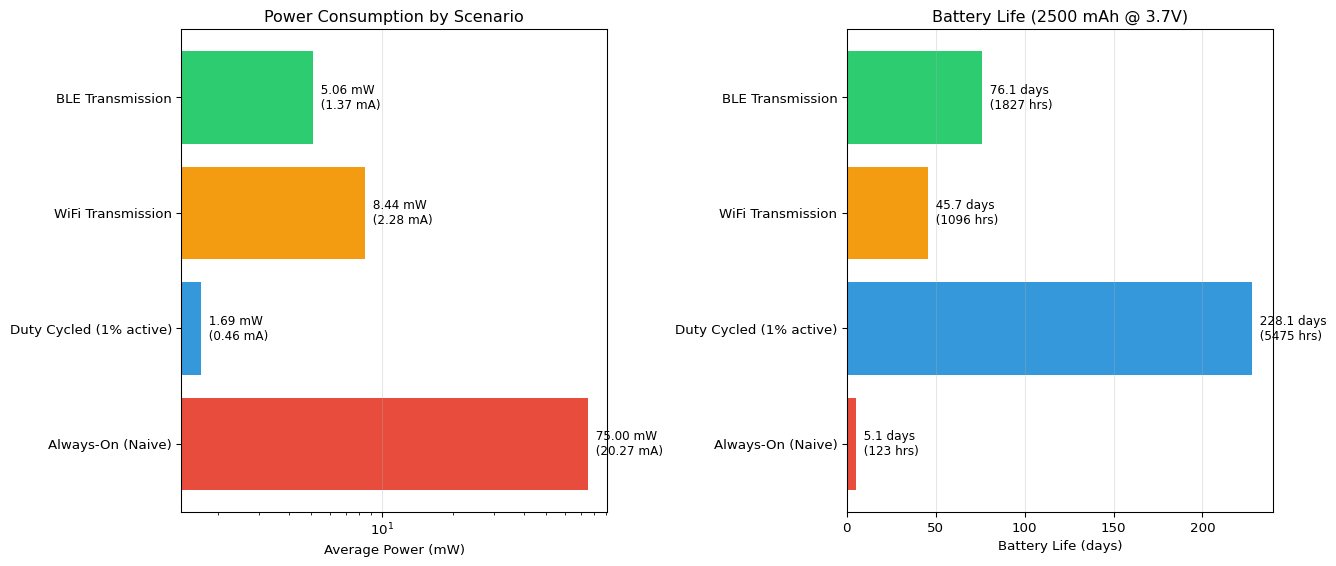

Energy Consumption Analysis
================================================================================
Battery: 2500 mAh @ 3.7 V = 9250.0 mWh

               Scenario  Avg Power (mW)  Avg Current (mA)  Battery Life (hours)  Battery Life (days)
      Always-On (Naive)         75.0000         20.270270            123.333333             5.138889
Duty Cycled (1% active)          1.6896          0.456649           5474.668561           228.111190
      WiFi Transmission          8.4380          2.280541           1096.231334            45.676306
       BLE Transmission          5.0630          1.368378           1826.980051            76.124169

Duty Cycled (1% active) vs Always-On: 44.4× longer battery life

WiFi Transmission vs Always-On: 8.9× longer battery life

BLE Transmission vs Always-On: 14.8× longer battery life

================================================================================
Key Insights:
  • Deep sleep reduces power by ~1000× (160mW → 0.04mW)
  • WiFi TX dominates energy budget even at 1% duty cycle
  • BLE uses 14× less power than WiFi (25mW vs 350mW)
  • Duty cycling extends battery life from days to months

Example 2: Duty Cycle Battery Life Estimator

import numpy as np
import matplotlib.pyplot as plt

def estimate_battery_life(battery_mAh, voltage, wake_interval_sec,
                         active_time_sec, active_power_mW,
                         sleep_power_mW, num_days=30):
    """
    Estimate battery life with periodic wake/sleep cycles

    Args:
        battery_mAh: Battery capacity in mAh
        voltage: Operating voltage (V)
        wake_interval_sec: Time between wake events (seconds)
        active_time_sec: Duration of active period (seconds)
        active_power_mW: Power during active period (mW)
        sleep_power_mW: Power during sleep period (mW)
        num_days: Number of days to simulate

    Returns:
        Dictionary with simulation results
    """
    # Calculate duty cycles
    sleep_time_sec = wake_interval_sec - active_time_sec
    active_duty = active_time_sec / wake_interval_sec
    sleep_duty = sleep_time_sec / wake_interval_sec

    # Calculate average power and current
    avg_power_mW = (active_power_mW * active_duty) + (sleep_power_mW * sleep_duty)
    avg_current_mA = avg_power_mW / voltage

    # Calculate battery life
    battery_life_hours = battery_mAh / avg_current_mA
    battery_life_days = battery_life_hours / 24

    # Simulate energy consumption over time
    total_seconds = num_days * 24 * 3600
    time_points = np.arange(0, total_seconds, wake_interval_sec)

    energy_consumed = []
    cumulative_energy = 0

    for t in time_points:
        # Energy in one cycle (mWh)
        cycle_energy = ((active_power_mW * active_time_sec) +
                       (sleep_power_mW * sleep_time_sec)) / 3600
        cumulative_energy += cycle_energy
        energy_consumed.append(cumulative_energy)

    battery_capacity_mWh = battery_mAh * voltage

    return {
        'active_duty': active_duty,
        'sleep_duty': sleep_duty,
        'avg_power_mW': avg_power_mW,
        'avg_current_mA': avg_current_mA,
        'battery_life_hours': battery_life_hours,
        'battery_life_days': battery_life_days,
        'time_hours': time_points / 3600,
        'energy_consumed_mWh': np.array(energy_consumed),
        'battery_capacity_mWh': battery_capacity_mWh,
        'wake_count': len(time_points)
    }

# Scenario 1: Environmental sensor (wake every 60s)
sensor_60s = estimate_battery_life(
    battery_mAh=2500,
    voltage=3.7,
    wake_interval_sec=60,
    active_time_sec=2,  # 2 seconds active
    active_power_mW=200,  # CPU + sensor + processing
    sleep_power_mW=0.04,  # Deep sleep
    num_days=60
)

# Scenario 2: Wearable device (wake every 10s)
wearable_10s = estimate_battery_life(
    battery_mAh=300,  # Smaller battery
    voltage=3.7,
    wake_interval_sec=10,
    active_time_sec=0.5,  # 500ms active
    active_power_mW=150,
    sleep_power_mW=0.05,
    num_days=14
)

# Scenario 3: Camera trap (wake every 5 min)
camera_5min = estimate_battery_life(
    battery_mAh=5000,  # Large battery
    voltage=3.7,
    wake_interval_sec=300,
    active_time_sec=5,  # 5 seconds active
    active_power_mW=500,  # Camera + processing
    sleep_power_mW=0.03,
    num_days=180
)

# Visualization
fig, ((ax1, ax2), (ax3, ax4)) = plt.subplots(2, 2, figsize=(14, 10))

# Plot 1: Duty cycle visualization
scenarios = ['Sensor\n(60s cycle)', 'Wearable\n(10s cycle)', 'Camera\n(5min cycle)']
active_duties = [sensor_60s['active_duty'], wearable_10s['active_duty'],
                 camera_5min['active_duty']]
sleep_duties = [sensor_60s['sleep_duty'], wearable_10s['sleep_duty'],
                camera_5min['sleep_duty']]

x = np.arange(len(scenarios))
width = 0.35

ax1.bar(x - width/2, np.array(active_duties) * 100, width,
        label='Active', color='#e74c3c')
ax1.bar(x + width/2, np.array(sleep_duties) * 100, width,
        label='Sleep', color='#2ecc71')
ax1.set_ylabel('Duty Cycle (%)')
ax1.set_title('Active vs Sleep Duty Cycles')
ax1.set_xticks(x)
ax1.set_xticklabels(scenarios)
ax1.legend()
ax1.grid(True, alpha=0.3, axis='y')

# Add percentage labels
for i, (active, sleep) in enumerate(zip(active_duties, sleep_duties)):
    ax1.text(i - width/2, active*100, f'{active*100:.1f}%',
             ha='center', va='bottom', fontsize=9)
    ax1.text(i + width/2, sleep*100, f'{sleep*100:.1f}%',
             ha='center', va='bottom', fontsize=9)

# Plot 2: Average power consumption
avg_powers = [sensor_60s['avg_power_mW'], wearable_10s['avg_power_mW'],
              camera_5min['avg_power_mW']]

ax2.bar(scenarios, avg_powers, color=['#3498db', '#9b59b6', '#f39c12'])
ax2.set_ylabel('Average Power (mW)')
ax2.set_title('Average Power Consumption')
ax2.grid(True, alpha=0.3, axis='y')

for i, power in enumerate(avg_powers):
    ax2.text(i, power, f'{power:.2f} mW',
             ha='center', va='bottom', fontsize=9)

# Plot 3: Battery discharge curves
ax3.plot(sensor_60s['time_hours'] / 24,
         sensor_60s['energy_consumed_mWh'] / sensor_60s['battery_capacity_mWh'] * 100,
         label='Sensor (2500mAh)', linewidth=2)
ax3.plot(wearable_10s['time_hours'] / 24,
         wearable_10s['energy_consumed_mWh'] / wearable_10s['battery_capacity_mWh'] * 100,
         label='Wearable (300mAh)', linewidth=2)
ax3.plot(camera_5min['time_hours'] / 24,
         camera_5min['energy_consumed_mWh'] / camera_5min['battery_capacity_mWh'] * 100,
         label='Camera (5000mAh)', linewidth=2)

ax3.axhline(y=100, color='r', linestyle='--', linewidth=1, alpha=0.5)
ax3.set_xlabel('Time (days)')
ax3.set_ylabel('Battery Charge (%)')
ax3.set_title('Battery Discharge Over Time')
ax3.legend()
ax3.grid(True, alpha=0.3)
ax3.set_xlim([0, max(sensor_60s['time_hours'][-1] / 24, 60)])

# Plot 4: Battery life comparison
battery_lives = [sensor_60s['battery_life_days'],
                wearable_10s['battery_life_days'],
                camera_5min['battery_life_days']]

colors_life = ['#3498db', '#9b59b6', '#f39c12']
bars = ax4.barh(scenarios, battery_lives, color=colors_life)
ax4.set_xlabel('Battery Life (days)')
ax4.set_title('Estimated Battery Life')
ax4.grid(True, alpha=0.3, axis='x')

for i, (life, current) in enumerate(zip(battery_lives,
                                        [sensor_60s['avg_current_mA'],
                                         wearable_10s['avg_current_mA'],
                                         camera_5min['avg_current_mA']])):
    ax4.text(life, i, f'  {life:.0f} days\n  ({current:.2f} mA avg)',
             va='center', fontsize=9)

plt.tight_layout()
plt.show()

# Print detailed results
print("Duty Cycle Battery Life Analysis")
print("="*80)

for name, result, battery in [('Environmental Sensor', sensor_60s, 2500),
                               ('Wearable Device', wearable_10s, 300),
                               ('Camera Trap', camera_5min, 5000)]:
    print(f"\n{name}:")
    print(f"  Battery: {battery} mAh @ 3.7V")
    print(f"  Active duty: {result['active_duty']*100:.2f}% | "
          f"Sleep duty: {result['sleep_duty']*100:.2f}%")
    print(f"  Average power: {result['avg_power_mW']:.3f} mW")
    print(f"  Average current: {result['avg_current_mA']:.3f} mA")
    print(f"  Battery life: {result['battery_life_days']:.1f} days "
          f"({result['battery_life_hours']:.0f} hours)")
    print(f"  Wake events: {result['wake_count']:,} over simulation period")

print("\n" + "="*80)
print("Optimization Tips:")
print("  • Increase wake interval to reduce active duty cycle")
print("  • Minimize active time through efficient code and quantization")
print("  • Use deep sleep between wake events (not light sleep)")
print("  • Batch sensor readings to reduce wake frequency")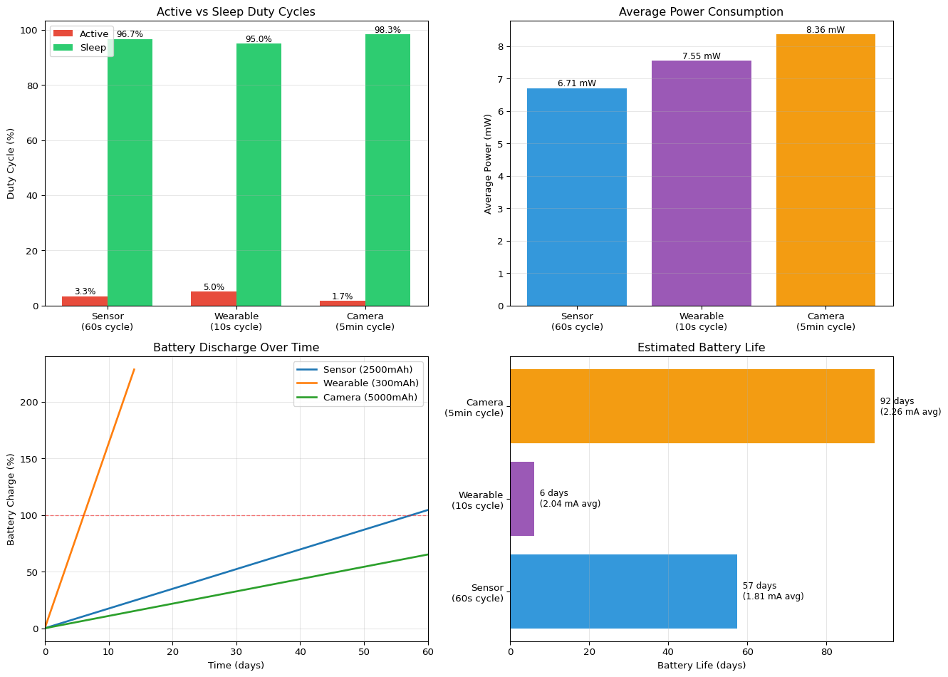

Duty Cycle Battery Life Analysis
================================================================================

Environmental Sensor:
  Battery: 2500 mAh @ 3.7V
  Active duty: 3.33% | Sleep duty: 96.67%
  Average power: 6.705 mW
  Average current: 1.812 mA
  Battery life: 57.5 days (1379 hours)
  Wake events: 86,400 over simulation period

Wearable Device:
  Battery: 300 mAh @ 3.7V
  Active duty: 5.00% | Sleep duty: 95.00%
  Average power: 7.548 mW
  Average current: 2.040 mA
  Battery life: 6.1 days (147 hours)
  Wake events: 120,960 over simulation period

Camera Trap:
  Battery: 5000 mAh @ 3.7V
  Active duty: 1.67% | Sleep duty: 98.33%
  Average power: 8.363 mW
  Average current: 2.260 mA
  Battery life: 92.2 days (2212 hours)
  Wake events: 51,840 over simulation period

================================================================================
Optimization Tips:
  • Increase wake interval to reduce active duty cycle
  • Minimize active time through efficient code and quantization
  • Use deep sleep between wake events (not light sleep)
  • Batch sensor readings to reduce wake frequency

Example 3: Power Profile Comparison

import numpy as np
import matplotlib.pyplot as plt

# Define power profiles for different operations
operations = {
    'Deep Sleep': 0.04,
    'Light Sleep': 0.8,
    'CPU Idle (20MHz)': 10,
    'CPU Active (80MHz)': 70,
    'CPU Active (160MHz)': 110,
    'CPU Active (240MHz)': 160,
    'Sensor Read': 15,
    'ML Inference (FP32)': 250,
    'ML Inference (INT8)': 80,
    'BLE Scan': 15,
    'BLE Connected': 25,
    'WiFi Scan': 150,
    'WiFi Connected': 100,
    'WiFi TX': 350,
}

# Create typical application profiles
profiles = {
    'Naive Design': [
        ('CPU Active (240MHz)', 1.0),
    ],
    'Frequency Optimized': [
        ('Deep Sleep', 0.70),
        ('CPU Active (80MHz)', 0.20),
        ('CPU Active (240MHz)', 0.10),
    ],
    'Quantized Model': [
        ('Deep Sleep', 0.95),
        ('Sensor Read', 0.02),
        ('ML Inference (INT8)', 0.02),
        ('BLE TX', 0.01),
    ],
    'Float32 Model': [
        ('Deep Sleep', 0.90),
        ('Sensor Read', 0.02),
        ('ML Inference (FP32)', 0.05),
        ('BLE TX', 0.03),
    ],
    'WiFi IoT Node': [
        ('Deep Sleep', 0.95),
        ('CPU Active (80MHz)', 0.03),
        ('Sensor Read', 0.01),
        ('WiFi TX', 0.01),
    ],
    'BLE Wearable': [
        ('Deep Sleep', 0.97),
        ('CPU Active (80MHz)', 0.02),
        ('Sensor Read', 0.005),
        ('BLE TX', 0.005),
    ],
}

# Calculate average power for each profile
profile_results = {}
for profile_name, components in profiles.items():
    total_power = sum(operations[op] * duty for op, duty in components)
    profile_results[profile_name] = {
        'power_mW': total_power,
        'current_mA': total_power / 3.7,
        'battery_life_days': 2500 / (total_power / 3.7) / 24,
        'components': components
    }

# Visualization
fig = plt.figure(figsize=(14, 10))
gs = fig.add_gridspec(3, 2, hspace=0.3, wspace=0.3)

# Plot 1: Power consumption comparison
ax1 = fig.add_subplot(gs[0, :])
profile_names = list(profile_results.keys())
powers = [profile_results[p]['power_mW'] for p in profile_names]
colors = plt.cm.viridis(np.linspace(0.2, 0.9, len(profile_names)))

bars = ax1.bar(profile_names, powers, color=colors, edgecolor='black', linewidth=1.5)
ax1.set_ylabel('Average Power (mW)', fontsize=12)
ax1.set_title('Power Consumption by Design Profile', fontsize=14, fontweight='bold')
ax1.set_yscale('log')
ax1.grid(True, alpha=0.3, axis='y')

# Annotate bars
for bar, power, current in zip(bars, powers,
                               [profile_results[p]['current_mA'] for p in profile_names]):
    height = bar.get_height()
    ax1.text(bar.get_x() + bar.get_width()/2, height,
             f'{power:.1f} mW\n({current:.2f} mA)',
             ha='center', va='bottom', fontsize=9)

plt.setp(ax1.xaxis.get_majorticklabels(), rotation=15, ha='right')

# Plot 2: Battery life comparison
ax2 = fig.add_subplot(gs[1, 0])
battery_lives = [profile_results[p]['battery_life_days'] for p in profile_names]

bars = ax2.barh(profile_names, battery_lives, color=colors,
                edgecolor='black', linewidth=1.5)
ax2.set_xlabel('Battery Life (days)', fontsize=12)
ax2.set_title('Battery Life (2500 mAh)', fontsize=12, fontweight='bold')
ax2.grid(True, alpha=0.3, axis='x')

for i, life in enumerate(battery_lives):
    ax2.text(life, i, f'  {life:.0f} days', va='center', fontsize=9)

# Plot 3: Component breakdown for quantized model
ax3 = fig.add_subplot(gs[1, 1])
quant_components = profiles['Quantized Model']
comp_names = [c[0] for c in quant_components]
comp_powers = [operations[c[0]] * c[1] for c in quant_components]

wedges, texts, autotexts = ax3.pie(comp_powers, labels=comp_names,
                                     autopct='%1.1f%%', startangle=90,
                                     colors=plt.cm.Set3(range(len(comp_names))))
ax3.set_title('Power Distribution:\nQuantized Model', fontsize=12, fontweight='bold')

# Plot 4: Comparison of ML inference methods
ax4 = fig.add_subplot(gs[2, 0])
ml_comparison = {
    'FP32 Inference': operations['ML Inference (FP32)'],
    'INT8 Inference': operations['ML Inference (INT8)'],
}

bars = ax4.bar(ml_comparison.keys(), ml_comparison.values(),
               color=['#e74c3c', '#2ecc71'], edgecolor='black', linewidth=1.5)
ax4.set_ylabel('Power (mW)', fontsize=12)
ax4.set_title('ML Inference Power Consumption', fontsize=12, fontweight='bold')
ax4.grid(True, alpha=0.3, axis='y')

# Add savings annotation
savings = (1 - operations['ML Inference (INT8)'] / operations['ML Inference (FP32)']) * 100
ax4.text(0.5, max(ml_comparison.values()) * 0.8,
         f'{savings:.0f}% Power Savings\nwith INT8 Quantization',
         ha='center', fontsize=11, bbox=dict(boxstyle='round', facecolor='wheat', alpha=0.5))

for bar, (name, power) in zip(bars, ml_comparison.items()):
    height = bar.get_height()
    ax4.text(bar.get_x() + bar.get_width()/2, height,
             f'{power:.0f} mW', ha='center', va='bottom', fontsize=10)

# Plot 5: Radio power comparison
ax5 = fig.add_subplot(gs[2, 1])
radio_comparison = {
    'WiFi TX': operations['WiFi TX'],
    'WiFi Connected': operations['WiFi Connected'],
    'BLE Connected': operations['BLE Connected'],
    'BLE Scan': operations['BLE Scan'],
}

bars = ax5.barh(list(radio_comparison.keys()), list(radio_comparison.values()),
                color=['#e74c3c', '#f39c12', '#2ecc71', '#3498db'],
                edgecolor='black', linewidth=1.5)
ax5.set_xlabel('Power (mW)', fontsize=12)
ax5.set_title('Radio Power Consumption', fontsize=12, fontweight='bold')
ax5.grid(True, alpha=0.3, axis='x')

for i, (name, power) in enumerate(radio_comparison.items()):
    ax5.text(power, i, f'  {power:.0f} mW', va='center', fontsize=9)

plt.tight_layout()
plt.show()

# Print detailed analysis
print("Power Profile Analysis")
print("="*80)
print(f"Battery: 2500 mAh @ 3.7V = 9250 mWh\n")

for profile_name in profile_names:
    result = profile_results[profile_name]
    print(f"{profile_name}:")
    print(f"  Average Power: {result['power_mW']:.2f} mW")
    print(f"  Average Current: {result['current_mA']:.2f} mA")
    print(f"  Battery Life: {result['battery_life_days']:.0f} days")
    print(f"  Components:")
    for op_name, duty in result['components']:
        power = operations[op_name] * duty
        print(f"    - {op_name}: {duty*100:.1f}% duty → {power:.3f} mW")
    print()

# Calculate improvements
baseline = profile_results['Naive Design']['battery_life_days']
print("="*80)
print("Optimization Impact (vs Naive Design):")
for profile_name in profile_names[1:]:
    improvement = profile_results[profile_name]['battery_life_days'] / baseline
    print(f"  {profile_name}: {improvement:.0f}× longer battery life")

KeyError: 'BLE TX'

Example 4: Energy per Inference Analysis

import numpy as np
import matplotlib.pyplot as plt

# Model characteristics
models = {
    'Tiny CNN': {
        'params': 8_000,
        'macs': 200_000,
        'accuracy': 96.8,
        'latency_ms_fp32': 12,
        'latency_ms_int8': 4,
        'power_mW_fp32': 200,
        'power_mW_int8': 60,
    },
    'Small CNN': {
        'params': 32_000,
        'macs': 800_000,
        'accuracy': 98.1,
        'latency_ms_fp32': 35,
        'latency_ms_int8': 10,
        'power_mW_fp32': 220,
        'power_mW_int8': 70,
    },
    'MobileNet': {
        'params': 125_000,
        'macs': 3_000_000,
        'accuracy': 98.9,
        'latency_ms_fp32': 120,
        'latency_ms_int8': 35,
        'power_mW_fp32': 250,
        'power_mW_int8': 80,
    },
    'ResNet-18': {
        'params': 11_000_000,
        'macs': 45_000_000,
        'accuracy': 99.2,
        'latency_ms_fp32': 850,
        'latency_ms_int8': 180,
        'power_mW_fp32': 300,
        'power_mW_int8': 95,
    },
}

# Calculate energy per inference
for model_name, specs in models.items():
    # Energy (mJ) = Power (mW) × Time (ms)
    specs['energy_mJ_fp32'] = specs['power_mW_fp32'] * specs['latency_ms_fp32']
    specs['energy_mJ_int8'] = specs['power_mW_int8'] * specs['latency_ms_int8']

    # Efficiency = Accuracy / Energy
    specs['efficiency_fp32'] = specs['accuracy'] / specs['energy_mJ_fp32']
    specs['efficiency_int8'] = specs['accuracy'] / specs['energy_mJ_int8']

# Visualization
fig, ((ax1, ax2), (ax3, ax4)) = plt.subplots(2, 2, figsize=(14, 10))

model_names = list(models.keys())
colors_fp32 = '#e74c3c'
colors_int8 = '#2ecc71'

# Plot 1: Energy per inference
energy_fp32 = [models[m]['energy_mJ_fp32'] for m in model_names]
energy_int8 = [models[m]['energy_mJ_int8'] for m in model_names]

x = np.arange(len(model_names))
width = 0.35

bars1 = ax1.bar(x - width/2, energy_fp32, width, label='FP32',
                color=colors_fp32, edgecolor='black')
bars2 = ax1.bar(x + width/2, energy_int8, width, label='INT8',
                color=colors_int8, edgecolor='black')

ax1.set_ylabel('Energy per Inference (mJ)', fontsize=11)
ax1.set_title('Energy Consumption: FP32 vs INT8', fontsize=12, fontweight='bold')
ax1.set_xticks(x)
ax1.set_xticklabels(model_names)
ax1.legend()
ax1.set_yscale('log')
ax1.grid(True, alpha=0.3, axis='y')

# Plot 2: Accuracy vs Energy (FP32)
ax2.scatter([models[m]['energy_mJ_fp32'] for m in model_names],
           [models[m]['accuracy'] for m in model_names],
           s=200, c=colors_fp32, alpha=0.6, edgecolors='black', linewidth=2)

for m in model_names:
    ax2.annotate(m, (models[m]['energy_mJ_fp32'], models[m]['accuracy']),
                xytext=(5, 5), textcoords='offset points', fontsize=9)

ax2.set_xlabel('Energy per Inference (mJ)', fontsize=11)
ax2.set_ylabel('Accuracy (%)', fontsize=11)
ax2.set_title('Accuracy vs Energy (FP32)', fontsize=12, fontweight='bold')
ax2.set_xscale('log')
ax2.grid(True, alpha=0.3)

# Plot 3: Accuracy vs Energy (INT8)
ax3.scatter([models[m]['energy_mJ_int8'] for m in model_names],
           [models[m]['accuracy'] for m in model_names],
           s=200, c=colors_int8, alpha=0.6, edgecolors='black', linewidth=2)

for m in model_names:
    ax3.annotate(m, (models[m]['energy_mJ_int8'], models[m]['accuracy']),
                xytext=(5, 5), textcoords='offset points', fontsize=9)

ax3.set_xlabel('Energy per Inference (mJ)', fontsize=11)
ax3.set_ylabel('Accuracy (%)', fontsize=11)
ax3.set_title('Accuracy vs Energy (INT8)', fontsize=12, fontweight='bold')
ax3.set_xscale('log')
ax3.grid(True, alpha=0.3)

# Plot 4: Efficiency comparison
efficiency_fp32 = [models[m]['efficiency_fp32'] for m in model_names]
efficiency_int8 = [models[m]['efficiency_int8'] for m in model_names]

bars1 = ax4.bar(x - width/2, efficiency_fp32, width, label='FP32',
                color=colors_fp32, edgecolor='black')
bars2 = ax4.bar(x + width/2, efficiency_int8, width, label='INT8',
                color=colors_int8, edgecolor='black')

ax4.set_ylabel('Efficiency (Accuracy % / mJ)', fontsize=11)
ax4.set_title('Energy Efficiency Comparison', fontsize=12, fontweight='bold')
ax4.set_xticks(x)
ax4.set_xticklabels(model_names)
ax4.legend()
ax4.grid(True, alpha=0.3, axis='y')

plt.tight_layout()
plt.show()

# Print detailed analysis
print("Energy per Inference Analysis")
print("="*80)

for model_name, specs in models.items():
    print(f"\n{model_name}:")
    print(f"  Parameters: {specs['params']:,}")
    print(f"  MACs: {specs['macs']:,}")
    print(f"  Accuracy: {specs['accuracy']:.1f}%")

    print(f"\n  FP32:")
    print(f"    Latency: {specs['latency_ms_fp32']:.0f} ms")
    print(f"    Power: {specs['power_mW_fp32']:.0f} mW")
    print(f"    Energy: {specs['energy_mJ_fp32']:.1f} mJ")
    print(f"    Efficiency: {specs['efficiency_fp32']:.3f} (acc%/mJ)")

    print(f"\n  INT8:")
    print(f"    Latency: {specs['latency_ms_int8']:.0f} ms")
    print(f"    Power: {specs['power_mW_int8']:.0f} mW")
    print(f"    Energy: {specs['energy_mJ_int8']:.1f} mJ")
    print(f"    Efficiency: {specs['efficiency_int8']:.3f} (acc%/mJ)")

    # Calculate speedup and energy savings
    speedup = specs['latency_ms_fp32'] / specs['latency_ms_int8']
    energy_savings = (1 - specs['energy_mJ_int8'] / specs['energy_mJ_fp32']) * 100
    efficiency_gain = (specs['efficiency_int8'] / specs['efficiency_fp32'] - 1) * 100

    print(f"\n  INT8 vs FP32:")
    print(f"    Speedup: {speedup:.1f}×")
    print(f"    Energy savings: {energy_savings:.1f}%")
    print(f"    Efficiency gain: {efficiency_gain:.1f}%")

# Calculate inferences per battery charge
battery_mWh = 2500 * 3.7  # 2500 mAh @ 3.7V
print("\n" + "="*80)
print(f"Inferences per Battery Charge (2500 mAh @ 3.7V = {battery_mWh:.0f} mWh):")
print("="*80)

for model_name in model_names:
    inferences_fp32 = battery_mWh / models[model_name]['energy_mJ_fp32']
    inferences_int8 = battery_mWh / models[model_name]['energy_mJ_int8']

    print(f"\n{model_name}:")
    print(f"  FP32: {inferences_fp32:,.0f} inferences")
    print(f"  INT8: {inferences_int8:,.0f} inferences ({inferences_int8/inferences_fp32:.1f}× more)")

print("\n" + "="*80)
print("Recommendation: For battery-powered edge devices,")
print("optimize for 'Accuracy per millijoule' rather than raw accuracy!")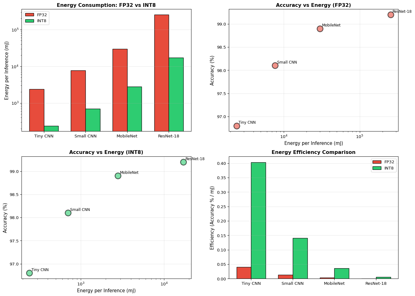

Energy per Inference Analysis
================================================================================

Tiny CNN:
  Parameters: 8,000
  MACs: 200,000
  Accuracy: 96.8%

  FP32:
    Latency: 12 ms
    Power: 200 mW
    Energy: 2400.0 mJ
    Efficiency: 0.040 (acc%/mJ)

  INT8:
    Latency: 4 ms
    Power: 60 mW
    Energy: 240.0 mJ
    Efficiency: 0.403 (acc%/mJ)

  INT8 vs FP32:
    Speedup: 3.0×
    Energy savings: 90.0%
    Efficiency gain: 900.0%

Small CNN:
  Parameters: 32,000
  MACs: 800,000
  Accuracy: 98.1%

  FP32:
    Latency: 35 ms
    Power: 220 mW
    Energy: 7700.0 mJ
    Efficiency: 0.013 (acc%/mJ)

  INT8:
    Latency: 10 ms
    Power: 70 mW
    Energy: 700.0 mJ
    Efficiency: 0.140 (acc%/mJ)

  INT8 vs FP32:
    Speedup: 3.5×
    Energy savings: 90.9%
    Efficiency gain: 1000.0%

MobileNet:
  Parameters: 125,000
  MACs: 3,000,000
  Accuracy: 98.9%

  FP32:
    Latency: 120 ms
    Power: 250 mW
    Energy: 30000.0 mJ
    Efficiency: 0.003 (acc%/mJ)

  INT8:
    Latency: 35 ms
    Power: 80 mW
    Energy: 2800.0 mJ
    Efficiency: 0.035 (acc%/mJ)

  INT8 vs FP32:
    Speedup: 3.4×
    Energy savings: 90.7%
    Efficiency gain: 971.4%

ResNet-18:
  Parameters: 11,000,000
  MACs: 45,000,000
  Accuracy: 99.2%

  FP32:
    Latency: 850 ms
    Power: 300 mW
    Energy: 255000.0 mJ
    Efficiency: 0.000 (acc%/mJ)

  INT8:
    Latency: 180 ms
    Power: 95 mW
    Energy: 17100.0 mJ
    Efficiency: 0.006 (acc%/mJ)

  INT8 vs FP32:
    Speedup: 4.7×
    Energy savings: 93.3%
    Efficiency gain: 1391.2%

================================================================================
Inferences per Battery Charge (2500 mAh @ 3.7V = 9250 mWh):
================================================================================

Tiny CNN:
  FP32: 4 inferences
  INT8: 39 inferences (10.0× more)

Small CNN:
  FP32: 1 inferences
  INT8: 13 inferences (11.0× more)

MobileNet:
  FP32: 0 inferences
  INT8: 3 inferences (10.7× more)

ResNet-18:
  FP32: 0 inferences
  INT8: 1 inferences (14.9× more)

================================================================================
Recommendation: For battery-powered edge devices,
optimize for 'Accuracy per millijoule' rather than raw accuracy!

Related Resources

• Hardware Guide - Equipment needed for Level 3
• Troubleshooting - Common issues and solutions