For detailed theoretical foundations, mathematical proofs, and algorithm derivations, see Chapter 14: Anomaly Detection on Edge Devices in the PDF textbook.
The PDF chapter includes: - Complete statistical anomaly detection theory (Z-score, IQR, Grubbs) - Detailed mathematical foundations of K-means clustering - In-depth autoencoder architecture and reconstruction loss theory - Comprehensive analysis of detection thresholds and ROC curves - Theoretical trade-offs between detection accuracy and edge constraints
Explain when anomaly detection is more appropriate than supervised classification on edge devices
Implement lightweight statistical detectors (Z-score, moving averages) that fit on microcontrollers
Apply K-means and tiny autoencoders for unsupervised anomaly detection on Pi/ESP32-class devices
Tune thresholds to trade off false alarms vs missed anomalies under edge resource constraints
Theory Summary
What is Anomaly Detection?
Anomaly detection identifies observations that deviate significantly from expected patterns. Unlike supervised classification (which requires labeled examples of both normal and abnormal data), anomaly detection typically learns from normal data only and flags anything unusual. This is ideal for edge devices where:
You have abundant “normal” operation data but few or no examples of failures
Anomalies are rare, unpredictable, or constantly evolving (new failure modes)
Labeling all possible anomalies is impractical or impossible
Common edge use cases include predictive maintenance (unusual vibration = impending failure), security (abnormal sensor readings = intrusion), quality control (defective products), health monitoring (irregular heart rhythms), and smart building fault detection.
Method Selection for Resource Constraints
Different anomaly detection methods have vastly different resource requirements:
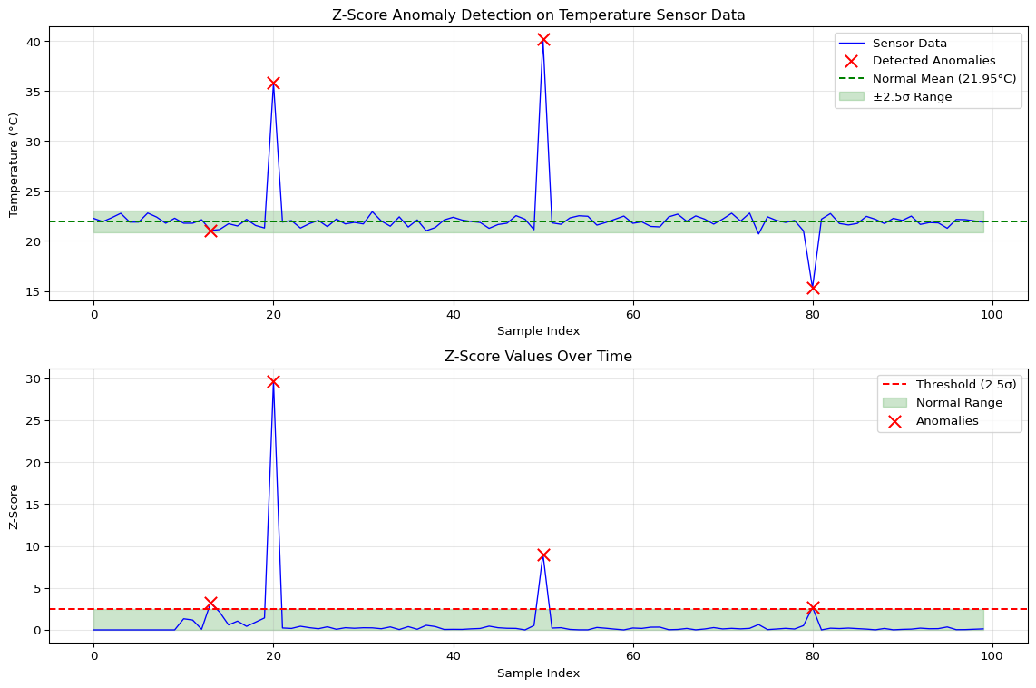
Z-Score (simplest, ~100 bytes memory, <1ms latency): Assumes data follows a normal distribution. Computes mean μ and standard deviation σ from training data, then flags values where |z| = |x - μ|/σ > threshold (typically 2-3). Perfect for Arduino-class MCUs with single-sensor monitoring.
Moving Average (~1KB memory): Maintains a sliding window of recent values. Detects anomalies when new values deviate significantly from the window average. Good for time-series data with slow drift.
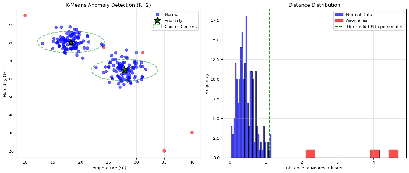
K-Means Clustering (~10KB memory, ~5ms latency): Finds K clusters in training data representing different “normal” operating modes (e.g., day/night, different load levels). Points far from all cluster centers are anomalies. Suitable for multi-dimensional data with multiple normal modes on ESP32 or Pi devices.
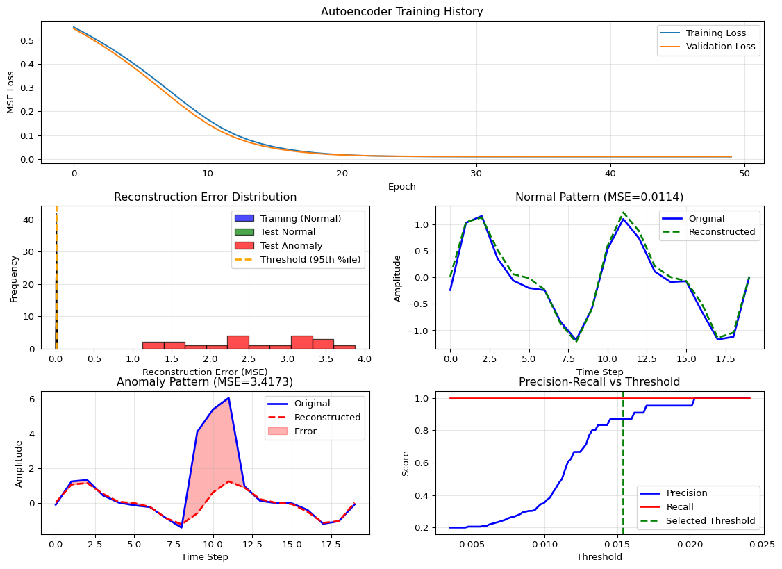
Autoencoder Neural Networks (~50KB+ memory, ~10ms+ latency): Learns to compress and reconstruct normal data. High reconstruction error indicates anomalies. Best for complex, non-linear patterns on Raspberry Pi or more capable devices. Tiny autoencoders can run on ESP32 with TFLite Micro.
Training and Threshold Selection
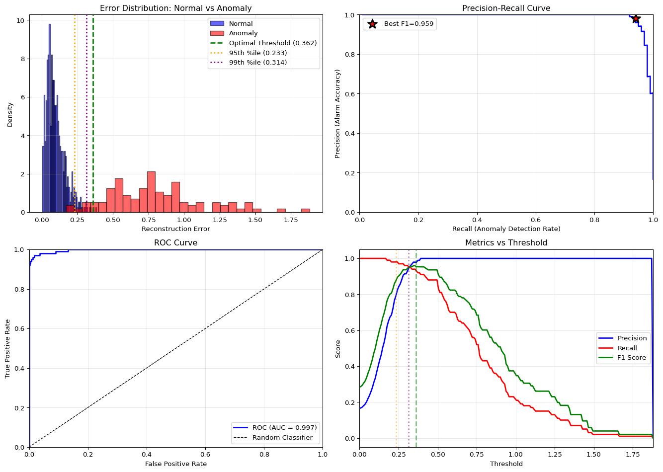
Critical rule: always train on normal data only. If you include anomalies in training, the model learns to reconstruct them, defeating the purpose. After training, set a threshold using the 95th-99th percentile of reconstruction error on normal validation data. This gives a baseline false positive rate of 1-5%.
The precision vs recall trade-off is application-specific: - High precision priority (minimize false alarms): Manufacturing quality control, non-critical alerts - High recall priority (don’t miss any anomalies): Safety systems, security, medical monitoring
Adjust the threshold accordingly: lower threshold = more sensitive but more false positives.
Key Concepts at a Glance
Core Concepts
Unsupervised Learning: Train on normal data only; no labels for anomalies required
Z-Score Formula: \(z = \frac{x - \mu}{\sigma}\), flag if \(|z| > threshold\) (typically 2-3)
Reconstruction Error: Autoencoders learn to reconstruct normal patterns; anomalies have high error
K-Means Distance: Points with distance > threshold from nearest cluster center are anomalies
Precision vs Recall: Precision = TP/(TP+FP) “accuracy of alarms”; Recall = TP/(TP+FN) “catch rate”
Never Poison Statistics: Don’t update mean/std with detected anomalies—they’ll corrupt the model
Common Pitfalls
Mistakes to Avoid
Using Z-Score on Non-Gaussian Data
Z-score assumes normal distribution. If your data is multimodal (e.g., sensor has day/night modes), Z-score produces many false positives. Always plot a histogram first. For multimodal data, use K-means with multiple clusters.
Training on Data Containing Anomalies
If anomalies sneak into training data, the model learns they’re “normal” and fails to detect future anomalies. Always verify training data is clean or use robust statistical methods that handle outliers.
Updating Statistics with Detected Anomalies
In the Arduino Z-score detector, only update mean/std when !isAnomaly. Otherwise, extreme values shift the baseline and future anomalies appear normal.
Setting Threshold Too High
Threshold = 3σ catches only 0.3% of normal data as false positives, but also misses subtle anomalies. Start with 2-2.5σ for most applications, then tune based on false positive rate.
Ignoring Concept Drift
Sensors drift over time (temperature, calibration changes). Use adaptive thresholds with exponential moving averages or periodic retraining to track gradual changes.
Quick Reference
Z-Score Detector (Arduino)
constint WINDOW_SIZE =50;constfloat THRESHOLD =2.5;float buffer[WINDOW_SIZE];int bufferIndex =0;int bufferCount =0;float runningSum =0;float runningSumSq =0;bool detectAnomaly(float value){// Calculate mean and std from running sumsfloat mean = runningSum / max(bufferCount,1);float variance =(runningSumSq / bufferCount)-(mean * mean);float std = sqrt(max(variance,0.0001));float z = abs(value - mean)/ std;bool isAnomaly =(bufferCount >=10)&&(z > THRESHOLD);// Only update with normal valuesif(!isAnomaly){if(bufferCount == WINDOW_SIZE){ runningSum -= buffer[bufferIndex]; runningSumSq -= buffer[bufferIndex]* buffer[bufferIndex];}else bufferCount++; runningSum += value; runningSumSq += value * value; buffer[bufferIndex]= value; bufferIndex =(bufferIndex +1)% WINDOW_SIZE;}return isAnomaly;}
Section 14.3: K-means clustering for multi-modal anomalies
Section 14.4: Autoencoder architecture and training procedures
Section 14.5: Threshold tuning and precision-recall trade-offs
Section 14.6: TFLite conversion for edge deployment
Self-Assessment Checkpoints
Test your understanding before proceeding to the exercises.
Question 1: Calculate the z-score for a sensor reading of 85 when the rolling window has mean=75 and std=5. Is this an anomaly with threshold=2.5?
Answer: z = |x - μ| / σ = |85 - 75| / 5 = 10 / 5 = 2.0. Since z = 2.0 < 2.5 (threshold), this is NOT flagged as an anomaly. The reading is exactly 2 standard deviations from the mean, which represents the 95th percentile (5% of normal values exceed this). With threshold=2.5, you only flag values beyond 2.5σ, capturing roughly the 99th percentile. Trade-off: lower threshold (e.g., 2.0) detects more anomalies but increases false positives; higher threshold (e.g., 3.0) reduces false alarms but might miss subtle anomalies.
Question 2: Why should you NEVER train an anomaly detector on data containing anomalies?
Answer: If anomalies are included in training data, the model learns they are “normal” and fails to detect future similar anomalies. Example: Training an autoencoder on vibration data that includes 5% faulty bearing samples teaches the network to reconstruct those fault patterns perfectly. Future faulty bearings have low reconstruction error and aren’t flagged. Solution: Always train on verified normal data only. After deployment, never update statistics (mean, std) when a sample is flagged as anomalous—otherwise anomalies gradually shift the baseline and future anomalies appear normal. Use if (!isAnomaly) { updateStatistics(); } pattern.
Question 3: Your sensor data has two distinct modes (day: mean=70°F, night: mean=55°F). Why does a single z-score detector fail?
Answer: Z-score assumes unimodal (single peak) Gaussian distribution. With bimodal data (day/night modes), normal daytime readings (70°F) are flagged as anomalies at night when mean=55°F (z = 3.0), and vice versa. This produces constant false positives. Solutions: (1) K-means with K=2 clusters: Learn separate statistics for each mode, flag points far from both clusters, (2) Time-aware thresholds: Maintain separate day/night statistics, (3) Moving window statistics: Use only recent data (last 2 hours) so statistics adapt to current mode. Always visualize histograms before choosing detection method—multimodal data needs clustering-based approaches.
Question 4: Compare memory requirements: Z-score vs K-means (K=3) vs tiny autoencoder for edge deployment.
Answer:Z-score: ~100 bytes (store mean, std, rolling buffer of 50 floats = 200 bytes). Fits on any Arduino. K-means (K=3, 5 features): ~500 bytes (3 centroids × 5 features × 4 bytes + distance calculations). Fits on ESP32 or Arduino with careful optimization. Tiny autoencoder (5→3→5): ~2KB model + ~10KB tensor arena = 12KB total. Requires ESP32 (520KB SRAM). Choose based on: (1) Data complexity (simple patterns → Z-score, multi-modal → K-means, non-linear → autoencoder), (2) Available memory (Arduino → Z-score, ESP32 → any), (3) Accuracy requirements (higher accuracy → more complex methods).
Question 5: Your anomaly detector has 95% precision but only 60% recall. Is this acceptable for a medical monitoring device?
Answer: No, this is dangerous for medical applications. Precision = 95% means only 5% of alarms are false positives (good), but Recall = 60% means you miss 40% of actual anomalies (bad). For critical safety applications (medical monitoring, industrial safety, security), high recall is essential—you cannot miss real anomalies even if it means more false alarms. Solution: Lower the anomaly threshold to increase recall to 90-95%, accepting higher false positive rate. Then add secondary verification (e.g., check multiple sensors, alert human operator). For non-critical applications (manufacturing quality, predictive maintenance), high precision may be acceptable to reduce alert fatigue. Tune threshold based on consequence of missed anomalies.
Interactive Notebook
The notebook below contains runnable code for all Level 1 activities.
Understand anomaly detection theory - statistical and ML approaches
Implement lightweight statistical methods for MCUs
Build autoencoder-based detectors for complex patterns
Evaluate with appropriate metrics for imbalanced data
Deploy anomaly detectors on resource-constrained devices
Prerequisites Check
Before You Begin
Make sure you have completed: - [ ] LAB 02: ML Foundations with TensorFlow - [ ] LAB 03: Model Quantization - [ ] Basic understanding of normal distributions
Part 1: Anomaly Detection Theory
1.1 What is an Anomaly?
An anomaly (outlier) is a data point that deviates significantly from expected behavior:
The reconstruction error threshold determines sensitivity:
\(\text{threshold} = \mu_{train} + k \cdot \sigma_{train}\)
Or use percentiles: - 95th percentile: Catches most anomalies, some false positives - 99th percentile: Fewer false positives, may miss subtle anomalies
Part 5: Method Comparison
Checkpoint: Self-Assessment
Knowledge Check
Before proceeding, make sure you can answer:
What is the Z-score formula and what does |z| > 3 mean?
Why is accuracy misleading for anomaly detection?
What’s the difference between precision and recall and which matters more?
Why train autoencoders on normal data only?
How do you select the reconstruction error threshold?
Experiment with different thresholds and window sizes, and document how they affect false positives vs false negatives.
Here you move from pure simulation to an edge-like node (laptop or Raspberry Pi) where you can prototype deployment decisions.
Take the trained autoencoder (or another suitable anomaly model) and convert it to TFLite.
Run inference on a Pi or laptop using the TFLite interpreter, feeding it:
real or recorded sensor streams from LAB12/13
or synthetic streams generated on-device.
Measure:
per-window inference time
model file size
basic memory usage (e.g., RSS or TFLite tensor arena where available).
Use these measurements plus your Level 1 results to decide which method(s) are viable on your target edge platform.
Deploy anomaly detection on real hardware.
Implement the Z-score detector from the chapter on an Arduino-class MCU reading a real sensor (e.g., temperature, vibration, light).
Tune thresholds on-device and observe behaviour:
how often does it flag anomalies in normal operation?
can it catch intentional “fault” injections (e.g., shaking a sensor, covering a light sensor)?
For more capable devices (ESP32/Pi), deploy the tiny autoencoder:
run it on a sliding window of sensor data
log reconstruction error and anomaly flags via Serial or network.
Optionally, connect this with LAB11/LAB15 by measuring latency and power impact of anomaly detection, and with LAB12/13 by sending only anomalies into the streaming/storage pipeline.
Related Labs
Unsupervised Learning & Detection
LAB02: ML Foundations - Supervised learning basics before anomalies
LAB12: Streaming - Apply anomaly detection to streaming data
LAB13: Distributed Data - Query and analyze stored data for anomalies
Edge Deployment
LAB03: Quantization - Optimize anomaly detectors for edge
2025-12-15 01:14:49.499239: I external/local_xla/xla/tsl/cuda/cudart_stub.cc:31] Could not find cuda drivers on your machine, GPU will not be used.
2025-12-15 01:14:49.544102: I tensorflow/core/platform/cpu_feature_guard.cc:210] This TensorFlow binary is optimized to use available CPU instructions in performance-critical operations.
To enable the following instructions: AVX2 FMA, in other operations, rebuild TensorFlow with the appropriate compiler flags.
2025-12-15 01:14:50.989716: I external/local_xla/xla/tsl/cuda/cudart_stub.cc:31] Could not find cuda drivers on your machine, GPU will not be used.
/opt/hostedtoolcache/Python/3.11.14/x64/lib/python3.11/site-packages/keras/src/layers/core/dense.py:95: UserWarning: Do not pass an `input_shape`/`input_dim` argument to a layer. When using Sequential models, prefer using an `Input(shape)` object as the first layer in the model instead.
  super().__init__(activity_regularizer=activity_regularizer, **kwargs)
2025-12-15 01:14:51.219864: E external/local_xla/xla/stream_executor/cuda/cuda_platform.cc:51] failed call to cuInit: INTERNAL: CUDA error: Failed call to cuInit: UNKNOWN ERROR (303)
/tmp/ipykernel_8945/3884694663.py:160: UserWarning: This figure includes Axes that are not compatible with tight_layout, so results might be incorrect.
  plt.tight_layout()
Autoencoder Anomaly Detection Results
============================================================
Model architecture: 20 → 8 → 4 → 8 → 20
Total parameters: 424
Model size (approx): ~1.66 KB (FP32)
Model size (INT8):   ~0.41 KB

Threshold: 0.0154

Performance Metrics:
  Precision: 0.870 (What % of alarms are real?)
  Recall:    1.000 (What % of anomalies caught?)
  F1 Score:  0.930

Detection Summary:
  True Positives:  20
  False Positives: 3
  True Negatives:  77
  False Negatives: 0
---title: "LAB14: Anomaly Detection"subtitle: "Unsupervised Learning on Edge"---::: {.callout-note}## PDF Textbook ReferenceFor detailed theoretical foundations, mathematical proofs, and algorithm derivations, see **Chapter 14: Anomaly Detection on Edge Devices** in the [PDF textbook](../downloads/Edge-Analytics-Lab-Book-v1.0.0.pdf).The PDF chapter includes:- Complete statistical anomaly detection theory (Z-score, IQR, Grubbs)- Detailed mathematical foundations of K-means clustering- In-depth autoencoder architecture and reconstruction loss theory- Comprehensive analysis of detection thresholds and ROC curves- Theoretical trade-offs between detection accuracy and edge constraints:::[](https://colab.research.google.com/github/ngcharithperera/edge-analytics-lab-book/blob/main/notebooks/LAB14_anomaly_detection.ipynb)[Download Notebook](https://raw.githubusercontent.com/ngcharithperera/edge-analytics-lab-book/main/notebooks/LAB14_anomaly_detection.ipynb)## Learning ObjectivesBy the end of this lab you should be able to:- Explain when anomaly detection is more appropriate than supervised classification on edge devices- Implement lightweight statistical detectors (Z-score, moving averages) that fit on microcontrollers- Apply K-means and tiny autoencoders for unsupervised anomaly detection on Pi/ESP32-class devices- Tune thresholds to trade off false alarms vs missed anomalies under edge resource constraints## Theory Summary### What is Anomaly Detection?Anomaly detection identifies observations that deviate significantly from expected patterns. Unlike supervised classification (which requires labeled examples of both normal and abnormal data), anomaly detection typically learns from normal data only and flags anything unusual. This is ideal for edge devices where:- You have abundant "normal" operation data but few or no examples of failures- Anomalies are rare, unpredictable, or constantly evolving (new failure modes)- Labeling all possible anomalies is impractical or impossibleCommon edge use cases include predictive maintenance (unusual vibration = impending failure), security (abnormal sensor readings = intrusion), quality control (defective products), health monitoring (irregular heart rhythms), and smart building fault detection.### Method Selection for Resource ConstraintsDifferent anomaly detection methods have vastly different resource requirements:**Z-Score** (simplest, ~100 bytes memory, <1ms latency): Assumes data follows a normal distribution. Computes mean μ and standard deviation σ from training data, then flags values where |z| = |x - μ|/σ > threshold (typically 2-3). Perfect for Arduino-class MCUs with single-sensor monitoring.**Moving Average** (~1KB memory): Maintains a sliding window of recent values. Detects anomalies when new values deviate significantly from the window average. Good for time-series data with slow drift.**K-Means Clustering** (~10KB memory, ~5ms latency): Finds K clusters in training data representing different "normal" operating modes (e.g., day/night, different load levels). Points far from all cluster centers are anomalies. Suitable for multi-dimensional data with multiple normal modes on ESP32 or Pi devices.**Autoencoder Neural Networks** (~50KB+ memory, ~10ms+ latency): Learns to compress and reconstruct normal data. High reconstruction error indicates anomalies. Best for complex, non-linear patterns on Raspberry Pi or more capable devices. Tiny autoencoders can run on ESP32 with TFLite Micro.### Training and Threshold SelectionCritical rule: **always train on normal data only**. If you include anomalies in training, the model learns to reconstruct them, defeating the purpose. After training, set a threshold using the 95th-99th percentile of reconstruction error on normal validation data. This gives a baseline false positive rate of 1-5%.The precision vs recall trade-off is application-specific:- **High precision priority** (minimize false alarms): Manufacturing quality control, non-critical alerts- **High recall priority** (don't miss any anomalies): Safety systems, security, medical monitoringAdjust the threshold accordingly: lower threshold = more sensitive but more false positives.## Key Concepts at a Glance::: {.callout-note icon=false}## Core Concepts- **Unsupervised Learning**: Train on normal data only; no labels for anomalies required- **Z-Score Formula**: $z = \frac{x - \mu}{\sigma}$, flag if $|z| > threshold$ (typically 2-3)- **Reconstruction Error**: Autoencoders learn to reconstruct normal patterns; anomalies have high error- **K-Means Distance**: Points with distance > threshold from nearest cluster center are anomalies- **Precision vs Recall**: Precision = TP/(TP+FP) "accuracy of alarms"; Recall = TP/(TP+FN) "catch rate"- **Never Poison Statistics**: Don't update mean/std with detected anomalies—they'll corrupt the model:::## Common Pitfalls::: {.callout-warning}## Mistakes to Avoid**Using Z-Score on Non-Gaussian Data**: Z-score assumes normal distribution. If your data is multimodal (e.g., sensor has day/night modes), Z-score produces many false positives. Always plot a histogram first. For multimodal data, use K-means with multiple clusters.**Training on Data Containing Anomalies**: If anomalies sneak into training data, the model learns they're "normal" and fails to detect future anomalies. Always verify training data is clean or use robust statistical methods that handle outliers.**Updating Statistics with Detected Anomalies**: In the Arduino Z-score detector, only update mean/std when `!isAnomaly`. Otherwise, extreme values shift the baseline and future anomalies appear normal.**Setting Threshold Too High**: Threshold = 3σ catches only 0.3% of normal data as false positives, but also misses subtle anomalies. Start with 2-2.5σ for most applications, then tune based on false positive rate.**Ignoring Concept Drift**: Sensors drift over time (temperature, calibration changes). Use adaptive thresholds with exponential moving averages or periodic retraining to track gradual changes.:::## Quick Reference### Z-Score Detector (Arduino)```cppconstint WINDOW_SIZE =50;constfloat THRESHOLD =2.5;float buffer[WINDOW_SIZE];int bufferIndex =0;int bufferCount =0;float runningSum =0;float runningSumSq =0;bool detectAnomaly(float value){// Calculate mean and std from running sumsfloat mean = runningSum / max(bufferCount,1);float variance =(runningSumSq / bufferCount)-(mean * mean);float std = sqrt(max(variance,0.0001));float z = abs(value - mean)/ std;bool isAnomaly =(bufferCount >=10)&&(z > THRESHOLD);// Only update with normal valuesif(!isAnomaly){if(bufferCount == WINDOW_SIZE){ runningSum -= buffer[bufferIndex]; runningSumSq -= buffer[bufferIndex]* buffer[bufferIndex];}else bufferCount++; runningSum += value; runningSumSq += value * value; buffer[bufferIndex]= value; bufferIndex =(bufferIndex +1)% WINDOW_SIZE;}return isAnomaly;}```### K-Means Detector (Python)```pythonfrom sklearn.cluster import KMeansimport numpy as np# Trainingkmeans = KMeans(n_clusters=3).fit(normal_data)distances = kmeans.transform(normal_data)min_distances = distances.min(axis=1)threshold = np.percentile(min_distances, 99) # 99th percentile# Detectiondef detect_kmeans_anomaly(point): distances = kmeans.transform([point])[0] min_distance = distances.min()return min_distance > threshold, min_distance```### Tiny Autoencoder (TensorFlow)```python# Training (normal data only!)autoencoder = tf.keras.Sequential([ tf.keras.layers.Dense(8, activation='relu', input_shape=(20,)), tf.keras.layers.Dense(4, activation='relu'), # Bottleneck tf.keras.layers.Dense(8, activation='relu'), tf.keras.layers.Dense(20, activation='linear')])autoencoder.compile(optimizer='adam', loss='mse')autoencoder.fit(normal_sequences, normal_sequences, epochs=50)# Set threshold from training errortrain_mse = np.mean((normal_sequences - autoencoder.predict(normal_sequences))**2, axis=1)threshold = np.percentile(train_mse, 95)# Detectiondef detect_autoencoder_anomaly(sequence): reconstruction = autoencoder.predict([sequence]) mse = np.mean((sequence - reconstruction)**2)return mse > threshold, mse```### Method Comparison Table| Method | Memory | Latency | Complexity | Best For ||--------|--------|---------|------------|----------|| **Z-Score** | ~100 B | <1 ms | Very Low | Arduino, single sensor || **Moving Avg** | ~1 KB | <1 ms | Low | Time series trends || **K-Means** | ~10 KB | ~5 ms | Medium | Multi-dimensional, multiple modes || **Autoencoder** | ~50 KB | ~10 ms | Higher | Complex non-linear patterns |### Evaluation Metrics$$\text{Precision} = \frac{TP}{TP + FP} \quad \text{(What \% of alarms are real?)}$$$$\text{Recall} = \frac{TP}{TP + FN} \quad \text{(What \% of anomalies caught?)}$$$$\text{F1 Score} = \frac{2 \times Precision \times Recall}{Precision + Recall}$$**Trade-off Example**: Manufacturing QC prioritizes precision (minimize false alarms that stop production). Security systems prioritize recall (catch all intrusions, tolerate false alarms).---::: {.callout-tip}## Related Concepts in PDF Chapter 14- Section 14.2: Statistical methods (Z-score, moving average) implementations- Section 14.3: K-means clustering for multi-modal anomalies- Section 14.4: Autoencoder architecture and training procedures- Section 14.5: Threshold tuning and precision-recall trade-offs- Section 14.6: TFLite conversion for edge deployment:::## Self-Assessment CheckpointsTest your understanding before proceeding to the exercises.::: {.callout-note collapse="true" title="Question 1: Calculate the z-score for a sensor reading of 85 when the rolling window has mean=75 and std=5. Is this an anomaly with threshold=2.5?"}**Answer:** z = |x - μ| / σ = |85 - 75| / 5 = 10 / 5 = 2.0. Since z = 2.0 < 2.5 (threshold), this is NOT flagged as an anomaly. The reading is exactly 2 standard deviations from the mean, which represents the 95th percentile (5% of normal values exceed this). With threshold=2.5, you only flag values beyond 2.5σ, capturing roughly the 99th percentile. Trade-off: lower threshold (e.g., 2.0) detects more anomalies but increases false positives; higher threshold (e.g., 3.0) reduces false alarms but might miss subtle anomalies.:::::: {.callout-note collapse="true" title="Question 2: Why should you NEVER train an anomaly detector on data containing anomalies?"}**Answer:** If anomalies are included in training data, the model learns they are "normal" and fails to detect future similar anomalies. Example: Training an autoencoder on vibration data that includes 5% faulty bearing samples teaches the network to reconstruct those fault patterns perfectly. Future faulty bearings have low reconstruction error and aren't flagged. Solution: Always train on verified normal data only. After deployment, never update statistics (mean, std) when a sample is flagged as anomalous—otherwise anomalies gradually shift the baseline and future anomalies appear normal. Use `if (!isAnomaly) { updateStatistics(); }` pattern.:::::: {.callout-note collapse="true" title="Question 3: Your sensor data has two distinct modes (day: mean=70°F, night: mean=55°F). Why does a single z-score detector fail?"}**Answer:** Z-score assumes unimodal (single peak) Gaussian distribution. With bimodal data (day/night modes), normal daytime readings (70°F) are flagged as anomalies at night when mean=55°F (z = 3.0), and vice versa. This produces constant false positives. Solutions: (1) **K-means with K=2 clusters**: Learn separate statistics for each mode, flag points far from both clusters, (2) **Time-aware thresholds**: Maintain separate day/night statistics, (3) **Moving window statistics**: Use only recent data (last 2 hours) so statistics adapt to current mode. Always visualize histograms before choosing detection method—multimodal data needs clustering-based approaches.:::::: {.callout-note collapse="true" title="Question 4: Compare memory requirements: Z-score vs K-means (K=3) vs tiny autoencoder for edge deployment."}**Answer:** **Z-score**: ~100 bytes (store mean, std, rolling buffer of 50 floats = 200 bytes). Fits on any Arduino. **K-means (K=3, 5 features)**: ~500 bytes (3 centroids × 5 features × 4 bytes + distance calculations). Fits on ESP32 or Arduino with careful optimization. **Tiny autoencoder (5→3→5)**: ~2KB model + ~10KB tensor arena = 12KB total. Requires ESP32 (520KB SRAM). Choose based on: (1) Data complexity (simple patterns → Z-score, multi-modal → K-means, non-linear → autoencoder), (2) Available memory (Arduino → Z-score, ESP32 → any), (3) Accuracy requirements (higher accuracy → more complex methods).:::::: {.callout-note collapse="true" title="Question 5: Your anomaly detector has 95% precision but only 60% recall. Is this acceptable for a medical monitoring device?"}**Answer:** No, this is dangerous for medical applications. **Precision = 95%** means only 5% of alarms are false positives (good), but **Recall = 60%** means you miss 40% of actual anomalies (bad). For critical safety applications (medical monitoring, industrial safety, security), high recall is essential—you cannot miss real anomalies even if it means more false alarms. Solution: Lower the anomaly threshold to increase recall to 90-95%, accepting higher false positive rate. Then add secondary verification (e.g., check multiple sensors, alert human operator). For non-critical applications (manufacturing quality, predictive maintenance), high precision may be acceptable to reduce alert fatigue. Tune threshold based on consequence of missed anomalies.:::## Interactive NotebookThe notebook below contains runnable code for all Level 1 activities.{{< embed ../../notebooks/LAB14_anomaly_detection.ipynb >}}## Three-Tier Activities::: {.panel-tabset}### Level 1: NotebookEnvironment: local Jupyter or Colab, no hardware required.Suggested workflow:1. Use the notebook to generate or load time-series sensor data (or reuse streams from LAB12).2. Implement and compare Z-score, K-means, and autoencoder-based anomaly detectors on the same dataset.3. For each method, measure: - precision, recall, and F1 - approximate memory footprint (parameters + buffers) - approximate per-sample or per-window latency.4. Experiment with different thresholds and window sizes, and document how they affect false positives vs false negatives.### Level 2: SimulatorHere you move from pure simulation to an edge-like node (laptop or Raspberry Pi) where you can prototype deployment decisions.1. Take the trained autoencoder (or another suitable anomaly model) and convert it to TFLite.2. Run inference on a Pi or laptop using the TFLite interpreter, feeding it: - real or recorded sensor streams from LAB12/13 - or synthetic streams generated on-device.3. Measure: - per-window inference time - model file size - basic memory usage (e.g., RSS or TFLite tensor arena where available).4. Use these measurements plus your Level 1 results to decide which method(s) are viable on your target edge platform.### Level 3: DeviceDeploy anomaly detection on real hardware.1. Implement the Z-score detector from the chapter on an Arduino-class MCU reading a real sensor (e.g., temperature, vibration, light).2. Tune thresholds on-device and observe behaviour: - how often does it flag anomalies in normal operation? - can it catch intentional “fault” injections (e.g., shaking a sensor, covering a light sensor)?3. For more capable devices (ESP32/Pi), deploy the tiny autoencoder: - run it on a sliding window of sensor data - log reconstruction error and anomaly flags via Serial or network.4. Optionally, connect this with LAB11/LAB15 by measuring latency and power impact of anomaly detection, and with LAB12/13 by sending only anomalies into the streaming/storage pipeline.:::## Related Labs::: {.callout-tip}## Unsupervised Learning & Detection- **LAB02: ML Foundations** - Supervised learning basics before anomalies- **LAB12: Streaming** - Apply anomaly detection to streaming data- **LAB13: Distributed Data** - Query and analyze stored data for anomalies:::::: {.callout-tip}## Edge Deployment- **LAB03: Quantization** - Optimize anomaly detectors for edge- **LAB11: Profiling** - Measure anomaly detection performance- **LAB15: Energy Optimization** - Energy-efficient anomaly detection:::## Try It Yourself: Executable Python ExamplesBelow are interactive Python examples you can run directly in this Quarto document to explore anomaly detection techniques.### Example 1: Z-Score Anomaly Detector```{python}import numpy as npimport matplotlib.pyplot as plt# Generate normal sensor data with some anomaliesnp.random.seed(42)normal_data = np.random.normal(loc=22.0, scale=0.5, size=100)anomalies = np.array([35.8, 40.2, 15.3]) # Temperature anomaliesanomaly_indices = [20, 50, 80]# Insert anomaliesdata = normal_data.copy()for idx, anom inzip(anomaly_indices, anomalies): data[idx] = anom# Z-score anomaly detectiondef zscore_detector(data, threshold=2.5, window_size=50): anomaly_flags = [] z_scores = []for i inrange(len(data)):# Use sliding window for statistics start_idx =max(0, i - window_size) window = data[start_idx:i]iflen(window) <10: anomaly_flags.append(False) z_scores.append(0)continue mean = np.mean(window) std = np.std(window)# Calculate z-score z =abs(data[i] - mean) / (std +1e-8) z_scores.append(z)# Detect anomaly is_anomaly = z > threshold anomaly_flags.append(is_anomaly)return np.array(anomaly_flags), np.array(z_scores)# Run detectoranomaly_flags, z_scores = zscore_detector(data, threshold=2.5)# Visualizationfig, (ax1, ax2) = plt.subplots(2, 1, figsize=(12, 8))# Plot 1: Sensor data with anomalies markedax1.plot(data, 'b-', label='Sensor Data', linewidth=1)ax1.scatter(np.where(anomaly_flags)[0], data[anomaly_flags], c='red', s=100, marker='x', label='Detected Anomalies', zorder=5)ax1.axhline(y=np.mean(normal_data), color='g', linestyle='--', label=f'Normal Mean ({np.mean(normal_data):.2f}°C)')ax1.fill_between(range(len(data)), np.mean(normal_data) -2.5*np.std(normal_data), np.mean(normal_data) +2.5*np.std(normal_data), alpha=0.2, color='green', label='±2.5σ Range')ax1.set_xlabel('Sample Index')ax1.set_ylabel('Temperature (°C)')ax1.set_title('Z-Score Anomaly Detection on Temperature Sensor Data')ax1.legend()ax1.grid(True, alpha=0.3)# Plot 2: Z-scoresax2.plot(z_scores, 'b-', linewidth=1)ax2.axhline(y=2.5, color='r', linestyle='--', label='Threshold (2.5σ)')ax2.fill_between(range(len(z_scores)), 0, 2.5, alpha=0.2, color='green', label='Normal Range')ax2.scatter(np.where(anomaly_flags)[0], z_scores[anomaly_flags], c='red', s=100, marker='x', label='Anomalies', zorder=5)ax2.set_xlabel('Sample Index')ax2.set_ylabel('Z-Score')ax2.set_title('Z-Score Values Over Time')ax2.legend()ax2.grid(True, alpha=0.3)plt.tight_layout()plt.show()# Print insightsprint("Z-Score Anomaly Detection Results")print("="*60)print(f"Total samples: {len(data)}")print(f"Detected anomalies: {np.sum(anomaly_flags)}")print(f"Detection rate: {np.sum(anomaly_flags) /len(anomaly_indices) *100:.1f}%")print(f"\nAnomaly details:")for idx in np.where(anomaly_flags)[0]:print(f" Index {idx}: Value={data[idx]:.2f}°C, Z-score={z_scores[idx]:.2f}")print(f"\nMemory footprint: ~{50*4+16} bytes (50 floats + metadata)")```### Example 2: K-Means Clustering for Anomaly Detection```{python}import numpy as npimport matplotlib.pyplot as pltfrom sklearn.cluster import KMeansfrom sklearn.preprocessing import StandardScaler# Generate multi-modal sensor data (day/night modes)np.random.seed(42)n_samples =200# Day mode: higher temperature and humidityday_temp = np.random.normal(28, 2, n_samples //2)day_humidity = np.random.normal(65, 5, n_samples //2)# Night mode: lower temperature and humiditynight_temp = np.random.normal(18, 1.5, n_samples //2)night_humidity = np.random.normal(80, 4, n_samples //2)# Combine datanormal_data = np.column_stack([ np.concatenate([day_temp, night_temp]), np.concatenate([day_humidity, night_humidity])])# Add some anomaliesanomalies = np.array([ [40, 30], # Hot and dry [10, 95], # Cold and humid [35, 20], # Very hot and very dry])data = np.vstack([normal_data, anomalies])# K-means clustering (K=2 for day/night modes)scaler = StandardScaler()data_scaled = scaler.fit_transform(data)kmeans = KMeans(n_clusters=2, random_state=42, n_init=10)kmeans.fit(data_scaled[:n_samples]) # Train only on normal data# Calculate distances to nearest clusterdistances = kmeans.transform(data_scaled)min_distances = distances.min(axis=1)# Set threshold at 99th percentile of training datathreshold = np.percentile(min_distances[:n_samples], 99)# Detect anomaliesanomaly_flags = min_distances > threshold# Visualizationfig, (ax1, ax2) = plt.subplots(1, 2, figsize=(14, 6))# Plot 1: Scatter plot with clusterscolors = ['blue'ifnot flag else'red'for flag in anomaly_flags]ax1.scatter(data[:, 0], data[:, 1], c=colors, alpha=0.6, s=50)# Plot cluster centerscenters_original = scaler.inverse_transform(kmeans.cluster_centers_)ax1.scatter(centers_original[:, 0], centers_original[:, 1], c='green', s=300, marker='*', edgecolors='black', linewidths=2, label='Cluster Centers', zorder=5)# Add threshold circlesfor center in centers_original: circle = plt.Circle(center, threshold * scaler.scale_[0], color='green', fill=False, linestyle='--', linewidth=2, alpha=0.5) ax1.add_patch(circle)ax1.set_xlabel('Temperature (°C)')ax1.set_ylabel('Humidity (%)')ax1.set_title('K-Means Anomaly Detection (K=2)')ax1.legend(['Normal', 'Anomaly', 'Cluster Centers'])ax1.grid(True, alpha=0.3)# Plot 2: Distance distributionax2.hist(min_distances[:n_samples], bins=30, alpha=0.7, label='Normal Data', color='blue', edgecolor='black')ax2.hist(min_distances[n_samples:], bins=10, alpha=0.7, label='Anomalies', color='red', edgecolor='black')ax2.axvline(threshold, color='green', linestyle='--', linewidth=2, label=f'Threshold (99th percentile)')ax2.set_xlabel('Distance to Nearest Cluster')ax2.set_ylabel('Frequency')ax2.set_title('Distance Distribution')ax2.legend()ax2.grid(True, alpha=0.3)plt.tight_layout()plt.show()# Print insightsprint("K-Means Anomaly Detection Results")print("="*60)print(f"Number of clusters: {kmeans.n_clusters}")print(f"Total samples: {len(data)}")print(f"Detected anomalies: {np.sum(anomaly_flags)}")print(f"True anomalies: {len(anomalies)}")print(f"Detection rate: {np.sum(anomaly_flags[-len(anomalies):]) /len(anomalies) *100:.1f}%")print(f"\nCluster centers (original scale):")for i, center inenumerate(centers_original):print(f" Cluster {i+1}: Temp={center[0]:.2f}°C, Humidity={center[1]:.2f}%")print(f"\nThreshold: {threshold:.4f}")print(f"Memory footprint: ~{kmeans.n_clusters *2*4+100} bytes")```### Example 3: Autoencoder Anomaly Detection```{python}import numpy as npimport matplotlib.pyplot as pltfrom tensorflow import kerasfrom tensorflow.keras import layers# Generate normal sequential data (vibration patterns)np.random.seed(42)n_sequences =500sequence_length =20# Normal vibration pattern: sinusoidal with noisedef generate_normal_sequence(): t = np.linspace(0, 4*np.pi, sequence_length) signal = np.sin(t) + np.sin(2*t) *0.5 noise = np.random.normal(0, 0.1, sequence_length)return signal + noise# Anomalous pattern: spike or irregulardef generate_anomaly_sequence(): seq = generate_normal_sequence()# Add spike spike_pos = np.random.randint(5, 15) seq[spike_pos:spike_pos+3] += np.random.uniform(3, 5)return seq# Generate training data (normal only)train_sequences = np.array([generate_normal_sequence() for _ inrange(400)])# Generate test data (normal + anomalies)test_normal = np.array([generate_normal_sequence() for _ inrange(80)])test_anomalies = np.array([generate_anomaly_sequence() for _ inrange(20)])test_sequences = np.vstack([test_normal, test_anomalies])test_labels = np.array([0]*80+ [1]*20) # 0=normal, 1=anomaly# Build tiny autoencoderinput_dim = sequence_lengthencoding_dim =4autoencoder = keras.Sequential([ layers.Dense(8, activation='relu', input_shape=(input_dim,)), layers.Dense(encoding_dim, activation='relu'), # Bottleneck layers.Dense(8, activation='relu'), layers.Dense(input_dim, activation='linear')])autoencoder.compile(optimizer='adam', loss='mse')# Train on normal data onlyhistory = autoencoder.fit( train_sequences, train_sequences, epochs=50, batch_size=32, validation_split=0.1, verbose=0)# Calculate reconstruction errorstrain_reconstructions = autoencoder.predict(train_sequences, verbose=0)train_mse = np.mean((train_sequences - train_reconstructions)**2, axis=1)test_reconstructions = autoencoder.predict(test_sequences, verbose=0)test_mse = np.mean((test_sequences - test_reconstructions)**2, axis=1)# Set threshold at 95th percentile of training errorthreshold = np.percentile(train_mse, 95)# Detect anomaliespredictions = (test_mse > threshold).astype(int)# Calculate metricsfrom sklearn.metrics import precision_score, recall_score, f1_scoreprecision = precision_score(test_labels, predictions)recall = recall_score(test_labels, predictions)f1 = f1_score(test_labels, predictions)# Visualizationfig = plt.figure(figsize=(14, 10))gs = fig.add_gridspec(3, 2, hspace=0.3)# Plot 1: Training lossax1 = fig.add_subplot(gs[0, :])ax1.plot(history.history['loss'], label='Training Loss')ax1.plot(history.history['val_loss'], label='Validation Loss')ax1.set_xlabel('Epoch')ax1.set_ylabel('MSE Loss')ax1.set_title('Autoencoder Training History')ax1.legend()ax1.grid(True, alpha=0.3)# Plot 2: Reconstruction error distributionax2 = fig.add_subplot(gs[1, 0])ax2.hist(train_mse, bins=30, alpha=0.7, label='Training (Normal)', color='blue', edgecolor='black')ax2.hist(test_mse[test_labels==0], bins=20, alpha=0.7, label='Test Normal', color='green', edgecolor='black')ax2.hist(test_mse[test_labels==1], bins=10, alpha=0.7, label='Test Anomaly', color='red', edgecolor='black')ax2.axvline(threshold, color='orange', linestyle='--', linewidth=2, label=f'Threshold (95th %ile)')ax2.set_xlabel('Reconstruction Error (MSE)')ax2.set_ylabel('Frequency')ax2.set_title('Reconstruction Error Distribution')ax2.legend()ax2.grid(True, alpha=0.3)# Plot 3: Example normal reconstructionax3 = fig.add_subplot(gs[1, 1])normal_idx =5ax3.plot(test_sequences[normal_idx], 'b-', label='Original', linewidth=2)ax3.plot(test_reconstructions[normal_idx], 'g--', label='Reconstructed', linewidth=2)ax3.set_xlabel('Time Step')ax3.set_ylabel('Amplitude')ax3.set_title(f'Normal Pattern (MSE={test_mse[normal_idx]:.4f})')ax3.legend()ax3.grid(True, alpha=0.3)# Plot 4: Example anomaly reconstructionax4 = fig.add_subplot(gs[2, 0])anomaly_idx =85ax4.plot(test_sequences[anomaly_idx], 'b-', label='Original', linewidth=2)ax4.plot(test_reconstructions[anomaly_idx], 'r--', label='Reconstructed', linewidth=2)ax4.fill_between(range(sequence_length), test_sequences[anomaly_idx], test_reconstructions[anomaly_idx], alpha=0.3, color='red', label='Error')ax4.set_xlabel('Time Step')ax4.set_ylabel('Amplitude')ax4.set_title(f'Anomaly Pattern (MSE={test_mse[anomaly_idx]:.4f})')ax4.legend()ax4.grid(True, alpha=0.3)# Plot 5: ROC-style threshold analysisax5 = fig.add_subplot(gs[2, 1])thresholds = np.linspace(train_mse.min(), train_mse.max(), 100)precisions = []recalls = []for t in thresholds: preds = (test_mse > t).astype(int)if preds.sum() >0: precisions.append(precision_score(test_labels, preds, zero_division=0)) recalls.append(recall_score(test_labels, preds))else: precisions.append(1.0) recalls.append(0.0)ax5.plot(thresholds, precisions, 'b-', label='Precision', linewidth=2)ax5.plot(thresholds, recalls, 'r-', label='Recall', linewidth=2)ax5.axvline(threshold, color='green', linestyle='--', linewidth=2, label='Selected Threshold')ax5.set_xlabel('Threshold')ax5.set_ylabel('Score')ax5.set_title('Precision-Recall vs Threshold')ax5.legend()ax5.grid(True, alpha=0.3)plt.tight_layout()plt.show()# Print insightsprint("Autoencoder Anomaly Detection Results")print("="*60)print(f"Model architecture: {input_dim} → 8 → {encoding_dim} → 8 → {input_dim}")print(f"Total parameters: {autoencoder.count_params()}")print(f"Model size (approx): ~{autoencoder.count_params() *4/1024:.2f} KB (FP32)")print(f"Model size (INT8): ~{autoencoder.count_params() /1024:.2f} KB")print(f"\nThreshold: {threshold:.4f}")print(f"\nPerformance Metrics:")print(f" Precision: {precision:.3f} (What % of alarms are real?)")print(f" Recall: {recall:.3f} (What % of anomalies caught?)")print(f" F1 Score: {f1:.3f}")print(f"\nDetection Summary:")print(f" True Positives: {np.sum((predictions ==1) & (test_labels ==1))}")print(f" False Positives: {np.sum((predictions ==1) & (test_labels ==0))}")print(f" True Negatives: {np.sum((predictions ==0) & (test_labels ==0))}")print(f" False Negatives: {np.sum((predictions ==0) & (test_labels ==1))}")```### Example 4: Threshold Tuning Visualization```{python}import numpy as npimport matplotlib.pyplot as pltfrom sklearn.metrics import precision_recall_curve, roc_curve, auc# Simulate reconstruction errors for normal and anomaly datanp.random.seed(42)# Normal data: low reconstruction errornormal_errors = np.random.gamma(2, 0.05, 500)# Anomaly data: high reconstruction erroranomaly_errors = np.random.gamma(5, 0.15, 100)# Combine and create labelsall_errors = np.concatenate([normal_errors, anomaly_errors])true_labels = np.array([0]*500+ [1]*100) # 0=normal, 1=anomaly# Calculate precision-recall curveprecision, recall, pr_thresholds = precision_recall_curve(true_labels, all_errors)# Calculate ROC curvefpr, tpr, roc_thresholds = roc_curve(true_labels, all_errors)roc_auc = auc(fpr, tpr)# Calculate F1 scores for different thresholdsf1_scores =2* (precision[:-1] * recall[:-1]) / (precision[:-1] + recall[:-1] +1e-8)best_threshold_idx = np.argmax(f1_scores)best_threshold = pr_thresholds[best_threshold_idx]# Visualizationfig, ((ax1, ax2), (ax3, ax4)) = plt.subplots(2, 2, figsize=(14, 10))# Plot 1: Distribution of errorsax1.hist(normal_errors, bins=50, alpha=0.6, label='Normal', color='blue', edgecolor='black', density=True)ax1.hist(anomaly_errors, bins=30, alpha=0.6, label='Anomaly', color='red', edgecolor='black', density=True)ax1.axvline(best_threshold, color='green', linestyle='--', linewidth=2, label=f'Optimal Threshold ({best_threshold:.3f})')# Mark different threshold optionspercentile_95 = np.percentile(normal_errors, 95)percentile_99 = np.percentile(normal_errors, 99)ax1.axvline(percentile_95, color='orange', linestyle=':', linewidth=2, label=f'95th %ile ({percentile_95:.3f})')ax1.axvline(percentile_99, color='purple', linestyle=':', linewidth=2, label=f'99th %ile ({percentile_99:.3f})')ax1.set_xlabel('Reconstruction Error')ax1.set_ylabel('Density')ax1.set_title('Error Distribution: Normal vs Anomaly')ax1.legend()ax1.grid(True, alpha=0.3)# Plot 2: Precision-Recall curveax2.plot(recall[:-1], precision[:-1], 'b-', linewidth=2)ax2.scatter(recall[best_threshold_idx], precision[best_threshold_idx], s=200, c='red', marker='*', edgecolors='black', linewidths=2, label=f'Best F1={f1_scores[best_threshold_idx]:.3f}', zorder=5)ax2.set_xlabel('Recall (Anomaly Detection Rate)')ax2.set_ylabel('Precision (Alarm Accuracy)')ax2.set_title('Precision-Recall Curve')ax2.grid(True, alpha=0.3)ax2.legend()ax2.set_xlim([0, 1])ax2.set_ylim([0, 1])# Plot 3: ROC curveax3.plot(fpr, tpr, 'b-', linewidth=2, label=f'ROC (AUC = {roc_auc:.3f})')ax3.plot([0, 1], [0, 1], 'k--', linewidth=1, label='Random Classifier')ax3.set_xlabel('False Positive Rate')ax3.set_ylabel('True Positive Rate')ax3.set_title('ROC Curve')ax3.grid(True, alpha=0.3)ax3.legend()ax3.set_xlim([0, 1])ax3.set_ylim([0, 1])# Plot 4: Metrics vs Thresholdtest_thresholds = np.linspace(all_errors.min(), all_errors.max(), 200)test_precision = []test_recall = []test_f1 = []for thresh in test_thresholds: predictions = (all_errors > thresh).astype(int) tp = np.sum((predictions ==1) & (true_labels ==1)) fp = np.sum((predictions ==1) & (true_labels ==0)) fn = np.sum((predictions ==0) & (true_labels ==1)) prec = tp / (tp + fp) if (tp + fp) >0else0 rec = tp / (tp + fn) if (tp + fn) >0else0 f1 =2* prec * rec / (prec + rec) if (prec + rec) >0else0 test_precision.append(prec) test_recall.append(rec) test_f1.append(f1)ax4.plot(test_thresholds, test_precision, 'b-', label='Precision', linewidth=2)ax4.plot(test_thresholds, test_recall, 'r-', label='Recall', linewidth=2)ax4.plot(test_thresholds, test_f1, 'g-', label='F1 Score', linewidth=2)ax4.axvline(best_threshold, color='green', linestyle='--', linewidth=2, alpha=0.5)ax4.axvline(percentile_95, color='orange', linestyle=':', linewidth=2, alpha=0.5)ax4.axvline(percentile_99, color='purple', linestyle=':', linewidth=2, alpha=0.5)ax4.set_xlabel('Threshold')ax4.set_ylabel('Score')ax4.set_title('Metrics vs Threshold')ax4.legend()ax4.grid(True, alpha=0.3)ax4.set_xlim([0, max(test_thresholds)])plt.tight_layout()plt.show()# Print comprehensive insightsprint("Threshold Tuning Analysis")print("="*60)print(f"Dataset: {len(normal_errors)} normal, {len(anomaly_errors)} anomalies")print(f"\nThreshold Options:")print(f" 95th percentile: {percentile_95:.4f}")print(f" 99th percentile: {percentile_99:.4f}")print(f" Optimal (max F1): {best_threshold:.4f}")# Evaluate each thresholdfor name, thresh in [("95th %ile", percentile_95), ("99th %ile", percentile_99), ("Optimal", best_threshold)]: preds = (all_errors > thresh).astype(int) tp = np.sum((preds ==1) & (true_labels ==1)) fp = np.sum((preds ==1) & (true_labels ==0)) fn = np.sum((preds ==0) & (true_labels ==1)) tn = np.sum((preds ==0) & (true_labels ==0)) prec = tp / (tp + fp) if (tp + fp) >0else0 rec = tp / (tp + fn) if (tp + fn) >0else0 f1 =2* prec * rec / (prec + rec) if (prec + rec) >0else0print(f"\n{name} Threshold ({thresh:.4f}):")print(f" Precision: {prec:.3f} Recall: {rec:.3f} F1: {f1:.3f}")print(f" TP={tp}, FP={fp}, TN={tn}, FN={fn}")print(f"\nRecommendations:")print(f" • Safety-critical (high recall): Use {percentile_95:.4f} (95th %ile)")print(f" • Balanced: Use {best_threshold:.4f} (max F1)")print(f" • Low false alarms (high prec): Use {percentile_99:.4f} (99th %ile)")```## Related Resources- [Hardware Guide](../resources/hardware.qmd) - Equipment needed for Level 3- [Troubleshooting](../resources/troubleshooting.qmd) - Common issues and solutions